Chapter 8 Aggregate Demand Aggregate Supply and the


- Slides: 39

Chapter 8 Aggregate Demand, Aggregate Supply, and the Great Depression Copyright © 2012 Pearson Addison-Wesley. All rights reserved.

• Combining aggregate demand with aggregate supply • So far we assumed that the price level is fixed. It means that changes in Y are calculated as: ∆Y = ∆AD/P; where P is fixed • Now we will drop this assumption. If P increases we have inflation, if P decreases we have deflation. When AD changes we can’t tell whether this is due to changes in Y, P or both. For this reason we need to introduce the AD AS curves Copyright © 2012 Pearson Addison-Wesley. All rights reserved. 8 -2

o Short run AS o Shows the amount of output that business firms are willing to produce at different price levels. , holding constant the nominal wage rate o Long run AS o Shows the amount of output that business firms are willing to produce when nominal wage rate has fully adjusted to any change in P. • AD curve • Shows different combinations of price level and real output at which money and commodity markets are both in equilibrium. Copyright © 2012 Pearson Addison-Wesley. All rights reserved. 8 -3

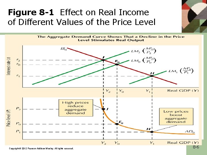
• Flexible prices and the AD curve. • Effects of changing prices on the LM curve. • LM shifts position whenever there is a change in real money supply, either due a change in nominal money supply, while P is fixed, or by a change in the price level, while nominal money supply remains fixed. • The upper part of the figure shows three values of P given fixed MS 0. Copyright © 2012 Pearson Addison-Wesley. All rights reserved. 8 -4

• If P were lower (p 1), real money supply will be higher. To maintain equilibrium in the money market r should fall to r 1 and Y to grow to Y 1. The reverse is true at higher price level. • • The lower part presents the relationship between Y and the assumed price level. Y along AD is always at a point where IS and LM cross, i. e. , along AD both the commodity and money markets are in equilibrium Copyright © 2012 Pearson Addison-Wesley. All rights reserved. 8 -5

Figure 8 -1 Effect on Real Income of Different Values of the Price Level Copyright © 2012 Pearson Addison-Wesley. All rights reserved. 8 -6

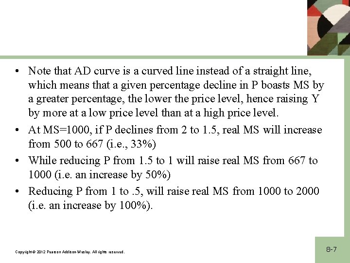
• Note that AD curve is a curved line instead of a straight line, which means that a given percentage decline in P boasts MS by a greater percentage, the lower the price level, hence raising Y by more at a low price level than at a high price level. • At MS=1000, if P declines from 2 to 1. 5, real MS will increase from 500 to 667 (i. e. , 33%) • While reducing P from 1. 5 to 1 will raise real MS from 667 to 1000 (i. e. an increase by 50%) • Reducing P from 1 to. 5, will raise real MS from 1000 to 2000 (i. e. an increase by 100%). Copyright © 2012 Pearson Addison-Wesley. All rights reserved. 8 -7

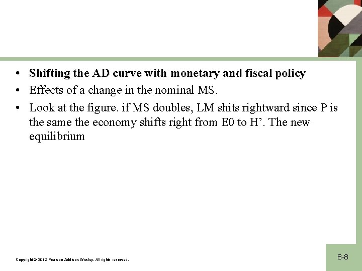
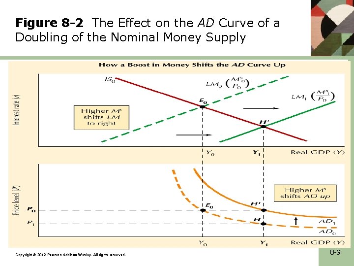
• Shifting the AD curve with monetary and fiscal policy • Effects of a change in the nominal MS. • Look at the figure. if MS doubles, LM shits rightward since P is the same the economy shifts right from E 0 to H’. The new equilibrium Copyright © 2012 Pearson Addison-Wesley. All rights reserved. 8 -8

Figure 8 -2 The Effect on the AD Curve of a Doubling of the Nominal Money Supply Copyright © 2012 Pearson Addison-Wesley. All rights reserved. 8 -9

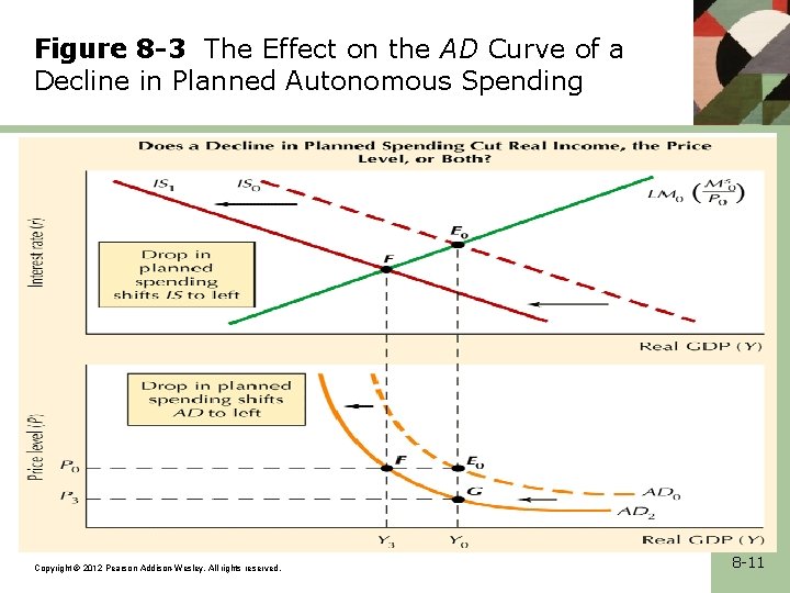
• Effects of a Change in Autonomous Spending • Now we assume that IS changes due to e. g. , a decline in business spending. • When IS shifts to the left, the position of the economy will shift to F if P is constant. Copyright © 2012 Pearson Addison-Wesley. All rights reserved. 8 -10

Figure 8 -3 The Effect on the AD Curve of a Decline in Planned Autonomous Spending Copyright © 2012 Pearson Addison-Wesley. All rights reserved. 8 -11

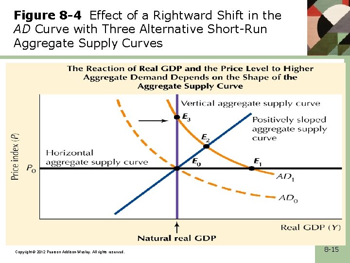
• Alternative shapes of the short run aggregates supply curve • How will the increase in AD be divided between higher Y. The answer will depend on AS, i. e. , whether it is horizontal, vertical or positively sloped. • Look at Figure 7 -4. Copyright © 2012 Pearson Addison-Wesley. All rights reserved. 8 -12

Aggregate Supply • The Short-Run Aggregate Supply (SAS) curve shows the amount of output that business firms are willing to produce at different price levels, holding constant the nominal wage rate – The SAS curve is upward sloping since an increase in the price level will increase profits for firms assuming wages and other input costs are fixed. This results in firms increasing output at higher prices • The Long-Run Aggregate Supply (LAS) curve shows the amount that business firms are willing to produce when the nominal wage rate has fully adjusted to any changes in the price level Copyright © 2012 Pearson Addison-Wesley. All rights reserved. 8 -13

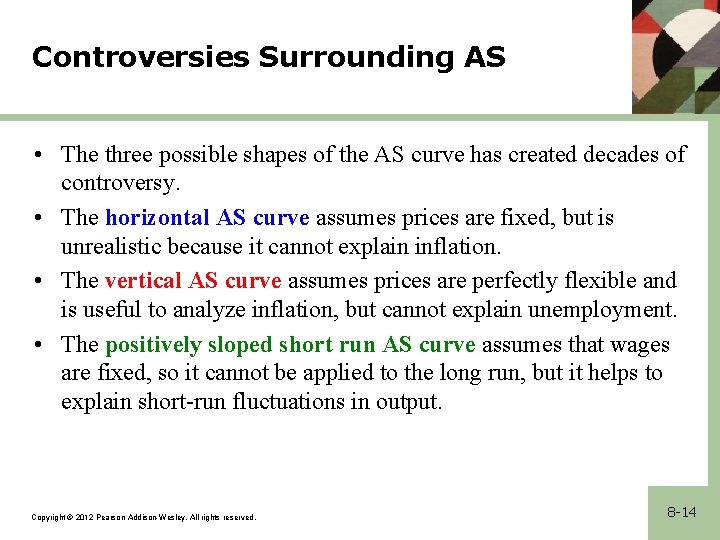
Controversies Surrounding AS • The three possible shapes of the AS curve has created decades of controversy. • The horizontal AS curve assumes prices are fixed, but is unrealistic because it cannot explain inflation. • The vertical AS curve assumes prices are perfectly flexible and is useful to analyze inflation, but cannot explain unemployment. • The positively sloped short run AS curve assumes that wages are fixed, so it cannot be applied to the long run, but it helps to explain short-run fluctuations in output. Copyright © 2012 Pearson Addison-Wesley. All rights reserved. 8 -14

Figure 8 -4 Effect of a Rightward Shift in the AD Curve with Three Alternative Short-Run Aggregate Supply Curves Copyright © 2012 Pearson Addison-Wesley. All rights reserved. 8 -15

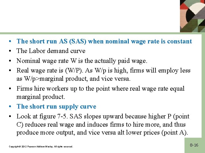
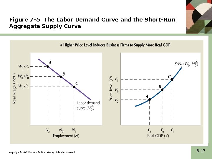
• • The short run AS (SAS) when nominal wage rate is constant The Labor demand curve Nominal wage rate W is the actually paid wage. Real wage rate is (W/P). As W/p is high, firms will employ less as W/p>marginal product, and vice versa. Firms hire workers up to the point where real wage rate equal marginal product. The short run supply curve Look at figure 7 -5. SAS slopes upward because higher P (point C) reduces real wage and induces firms to hire more, and thus produce more output, and vice versa alt lower prices (point A). Copyright © 2012 Pearson Addison-Wesley. All rights reserved. 8 -16

Figure 7 -5 The Labor Demand Curve and the Short-Run Aggregate Supply Curve Copyright © 2012 Pearson Addison-Wesley. All rights reserved. 8 -17

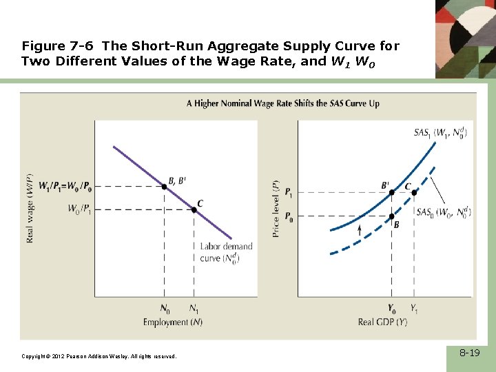
• How the wage rate is set • If wage rate increases, the SAS curve will shift up and its intersection point with AD will shift as well. Thus the determinants of the actual wage rate paid have a crucial effect on the nature of the economy’s response to a change in AD. • The equilibrium wage rate • In figure 7. 6. higher wage rate shifts the SAS curve because at a given price, workers are more costly and so firms hire fewer workers and produce less output. Point B and B’ are identical because we assume that the percentage difference between W 1 and W 0 is the save as between p 1 and p 0. thus point B’ lies directly above point B in the right frame. Copyright © 2012 Pearson Addison-Wesley. All rights reserved. 8 -18

Figure 7 -6 The Short-Run Aggregate Supply Curve for Two Different Values of the Wage Rate, and W 1 W 0 Copyright © 2012 Pearson Addison-Wesley. All rights reserved. 8 -19

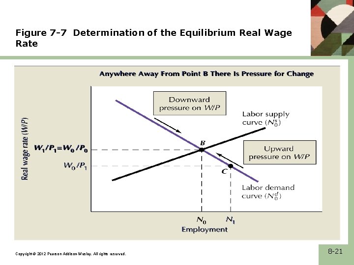
• Determinants of the equilibrium real wage rate • Equilibrium real wage rate is determined by the intersection of labor demand supply curves. Figure 7 -7. if firms are to raise employment to N 1 real wage rate must be reduced (at point C). • Employers need to find some factor that will make workers willing to provide more work than shown by their labor supply curve. Otherwise we would never observe changes in employment over the business cycle. • Labor contracts and wage bargaining • Contracts explain fixity of nominal wages in the short run. • If the economy operates above levels that are consistent with labor market equilibrium, firms and workers know that the real wage is reduced below equilibrium. Next change there will be an upward pressure on nominal wage rate to restore the equilibrium wage rate. Copyright © 2012 Pearson Addison-Wesley. All rights reserved. 8 -20

Figure 7 -7 Determination of the Equilibrium Real Wage Rate Copyright © 2012 Pearson Addison-Wesley. All rights reserved. 8 -21

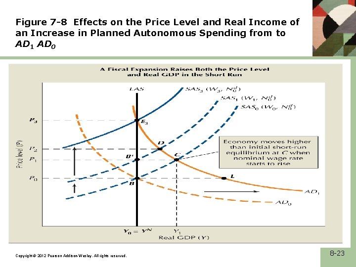
• Fiscal and monetary expansion in the short and long run • Initial short run effect of a fiscal expansion • Look at figure 7 -8. Initial fiscal stimulus shifts AD to AD 1, the economy shifts to point C. • The rising nominal wage and the arrival at long run equilibrium • Businesses are satisfied at point C but workers are not, as wage rate is the same. Workers would insist to increase nominal wage rate to W 1/P 1, but this is less than the equilibrium real wage rate. As they raise real wage rate, the economy slides to E 3. • The long run aggregate supply curve • LAS, the level of output YN is the labor market in equilibrium at the original real wage rate Copyright © 2012 Pearson Addison-Wesley. All rights reserved. 8 -22

Figure 7 -8 Effects on the Price Level and Real Income of an Increase in Planned Autonomous Spending from to AD 1 AD 0 Copyright © 2012 Pearson Addison-Wesley. All rights reserved. 8 -23

• Short run and long run equilibrium • Short run equilibrium occurs at the point where the AD crosses he SAS curve. • Long run equilibrium is a situation in which labor input is the amount voluntarily supplied and demanded at the equilibrium wage rate. Copyright © 2012 Pearson Addison-Wesley. All rights reserved. 8 -24

• Interpretation of the business cycle. • Note that in the short run prices are flexible while the wage rate is fixed. Price flexibility and wage fixity implies a countercyclical movement of the real wage rate, i. e. , movements of real wage rate are in the opposite direction of real GDP. (in reality movements are not in that manner) • An alternative view is that both prices and wages are fixed in the short run, and the SAS is relatively flat. When real GDP rises above equilibrium both prices and wage rise, and inflationary pressures continue until the economy returns to a point along the LAS (E 3). Copyright © 2012 Pearson Addison-Wesley. All rights reserved. 8 -25

• Classical macroeconomics: the quantity theory of money and the self correcting economy. • Classical economists believed that the economy possessed a powerful self correcting forces that guaranteed full employment and prevented Y from falling below YN for a long time. • these forces are flexible wages and prices that would adjust rapidly to absorb the impact of shifts in aggregate demand. • The quantity equation and the quantity theory of money MSV ≡ PY/MS • Changes in MS cause proportional changes in P. Note that V is assumed to be stable in the short run, and business cycles are attributed to changes in MS. Copyright © 2012 Pearson Addison-Wesley. All rights reserved. 8 -26

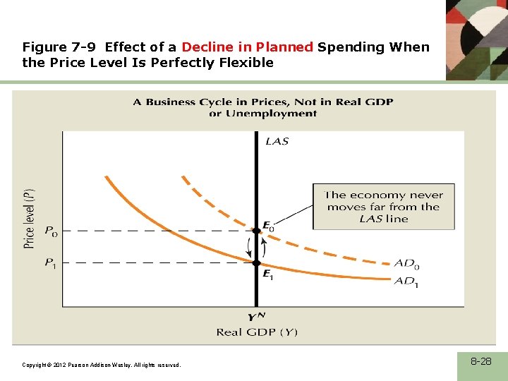
• Self correction in aggregate demand-supply model • Look at figure 7 -9. the classical economists assumed that the economy would not operate away from the LAS. No business cycle in Y would occur. • Classical view of unemployment and output fluctuations • Classical economists did not believe that Y could remain for more than short time below YN. How did they explain unemployment. Unemployed were described as irresponsible, or having an insufficient desire to work. Any unemployment will reduce real wage rate until equilibrium is obtained in the labor market. Copyright © 2012 Pearson Addison-Wesley. All rights reserved. 8 -27

Figure 7 -9 Effect of a Decline in Planned Spending When the Price Level Is Perfectly Flexible Copyright © 2012 Pearson Addison-Wesley. All rights reserved. 8 -28

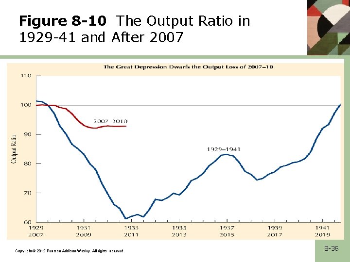
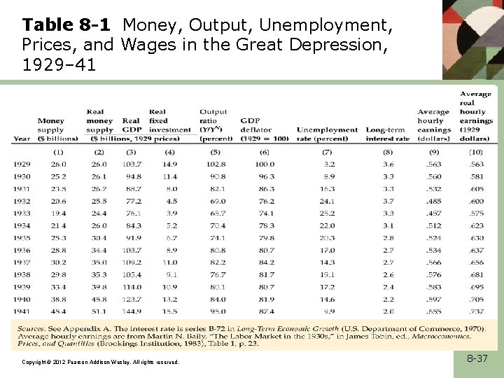
• The Keynesian revolution: the Failure of self correction. • The Great Depression of 1929 Y had declined by one third by 1932 and unemployment rose to more than 20%. It was time for a new diagnosis. This is presented by Keynes in 1936 and J. Hicks presented the IS-LM model a year later. • Monetary impotence and the failure of self correction in extreme cases • For Keynes the problem could be divided into two categories, one concerning demand due to the possibility of monetary impotence and the other concerning supply due to rigid wages Copyright © 2012 Pearson Addison-Wesley. All rights reserved. 8 -29

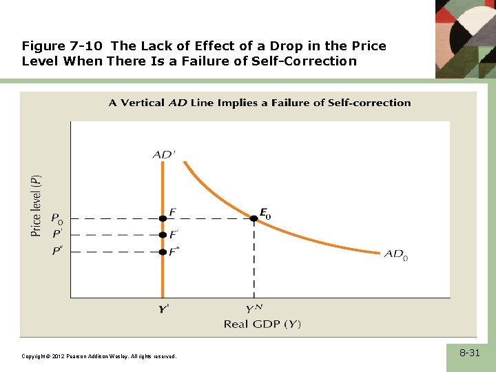
• Unresponsive expenditure: the vertical IS curve • If IS is vertical any change in MS will shift LM up or down a vertical IS curve, leaving Y unaffected. Look at figure 7 -10. If IS is vertical changes in P will have no effect on Y’. • The liquidity trap: A horizontal LM curve • If the LM is horizontal see figure 7 -10. if the IS intersects the LM in the horizontal section, an increase in MS/P does not shift the LM and Y stuck to Y’ where AD remains vertical. • Monetary impotence and a failure of self correction arise when there is a vertical IS or horizontal LM. The price level can fall to P” and Y remains at Y’. The economy would move from F to F’ or F” without any right word motion. Copyright © 2012 Pearson Addison-Wesley. All rights reserved. 8 -30

Figure 7 -10 The Lack of Effect of a Drop in the Price Level When There Is a Failure of Self-Correction Copyright © 2012 Pearson Addison-Wesley. All rights reserved. 8 -31

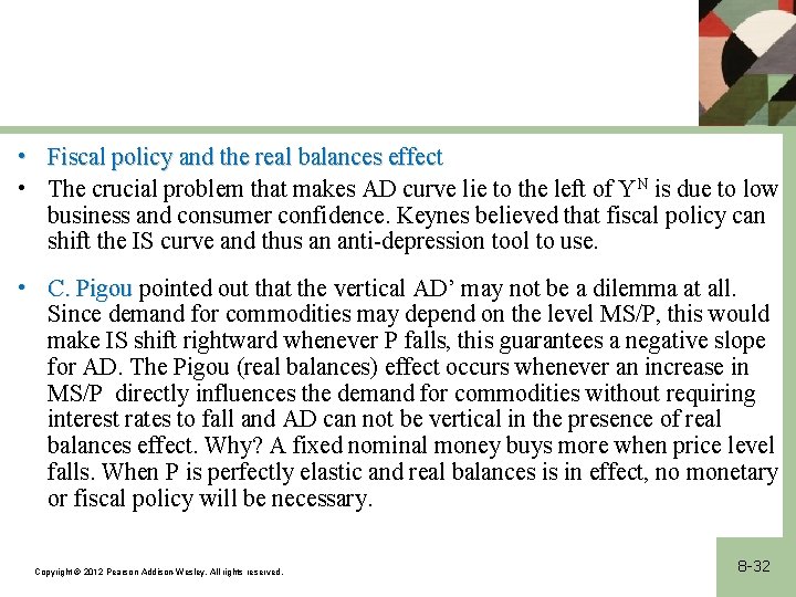
• Fiscal policy and the real balances effect • The crucial problem that makes AD curve lie to the left of YN is due to low business and consumer confidence. Keynes believed that fiscal policy can shift the IS curve and thus an anti-depression tool to use. • C. Pigou pointed out that the vertical AD’ may not be a dilemma at all. Since demand for commodities may depend on the level MS/P, this would make IS shift rightward whenever P falls, this guarantees a negative slope for AD. The Pigou (real balances) effect occurs whenever an increase in MS/P directly influences the demand for commodities without requiring interest rates to fall and AD can not be vertical in the presence of real balances effect. Why? A fixed nominal money buys more when price level falls. When P is perfectly elastic and real balances is in effect, no monetary or fiscal policy will be necessary. Copyright © 2012 Pearson Addison-Wesley. All rights reserved. 8 -32

• Two stimulative effects of price deflation. 1 - the Keynesian effect. An increase in C or I due to a decline in r either because of higher MS or lower P, both will increase MS/P. 2 - the Pigou effect. the direct stimulus to C when a price deflation causes an increase in MS/P. • • Destabilizing effects of falling prices Unfortunately the stimulative effects are not always favorable. There are two major unfavorable effects of deflation; 1. The expectation effect. People tend to postpone their purchases as the prices continue to decline. This may be strong enough to offset the stimulus of the Pigou effect. 8 -33 Copyright © 2012 Pearson Addison-Wesley. All rights reserved.

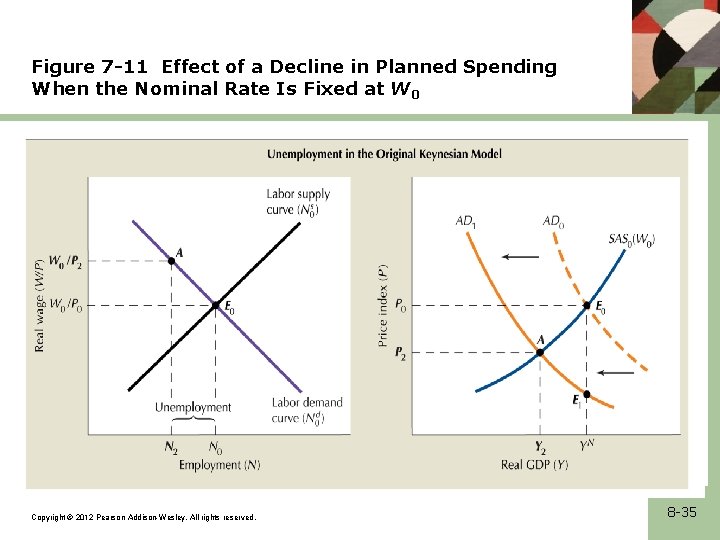
2. The redistribution effect. As unexpected deflation causes a redistribution of income from debtors to creditors, which reduces AD. • • Nominal wage rigidity Keynes’ second line of attack was simply that deflation would not occur in the necessary amount because of rigid nominal wages. Look at figure 7 -11. Keynes pointed out that the economy would remain stuck at point A even with the normally sloped AD curve AD 1. Copyright © 2012 Pearson Addison-Wesley. All rights reserved. 8 -34

Figure 7 -11 Effect of a Decline in Planned Spending When the Nominal Rate Is Fixed at W 0 Copyright © 2012 Pearson Addison-Wesley. All rights reserved. 8 -35

Figure 8 -10 The Output Ratio in 1929 -41 and After 2007 Copyright © 2012 Pearson Addison-Wesley. All rights reserved. 8 -36

Table 8 -1 Money, Output, Unemployment, Prices, and Wages in the Great Depression, 1929– 41 Copyright © 2012 Pearson Addison-Wesley. All rights reserved. 8 -37

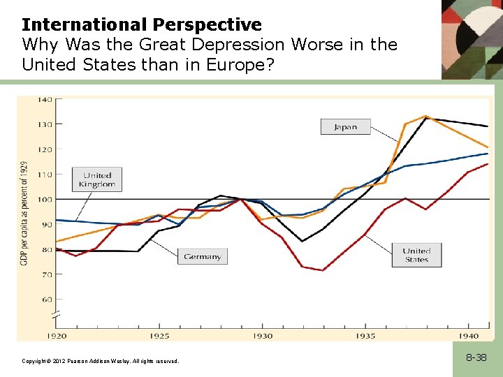
International Perspective Why Was the Great Depression Worse in the United States than in Europe? Copyright © 2012 Pearson Addison-Wesley. All rights reserved. 8 -38

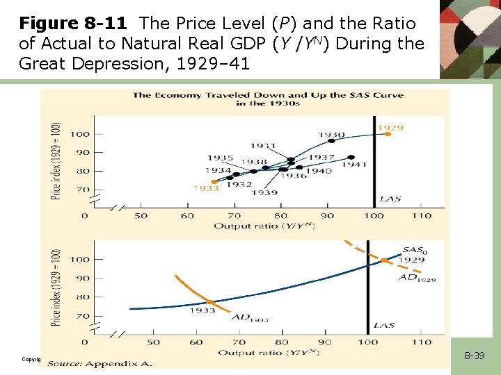
Figure 8 -11 The Price Level (P) and the Ratio of Actual to Natural Real GDP (Y /YN) During the Great Depression, 1929– 41 Copyright © 2012 Pearson Addison-Wesley. All rights reserved. 8 -39