Chapter 8 Aggregate Demand Aggregate Supply and the

- Slides: 25

Chapter 8 • Aggregate Demand, • Aggregate Supply, and the Great Depression Copyright © 2012 Pearson Addison-Wesley. All rights reserved.

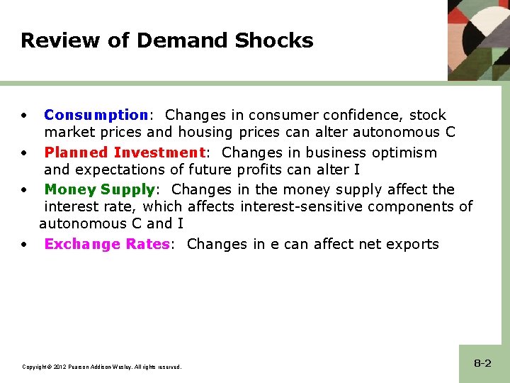
Review of Demand Shocks • Consumption: Changes in consumer confidence, stock market prices and housing prices can alter autonomous C • Planned Investment: Changes in business optimism and expectations of future profits can alter I • Money Supply: Changes in the money supply affect the interest rate, which affects interest-sensitive components of autonomous C and I • Exchange Rates: Changes in e can affect net exports Copyright © 2012 Pearson Addison-Wesley. All rights reserved. 8 -2

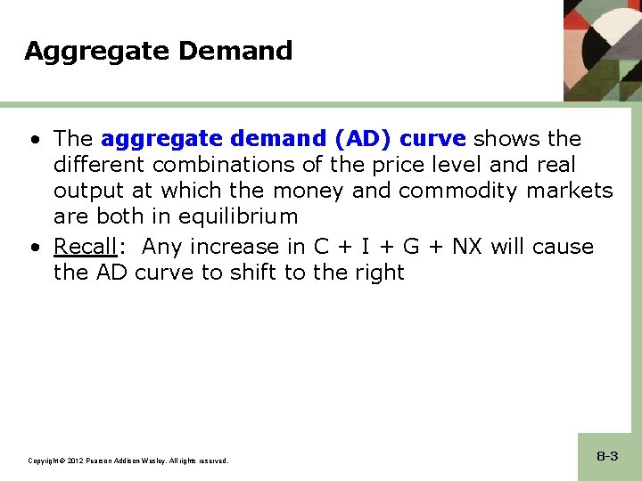
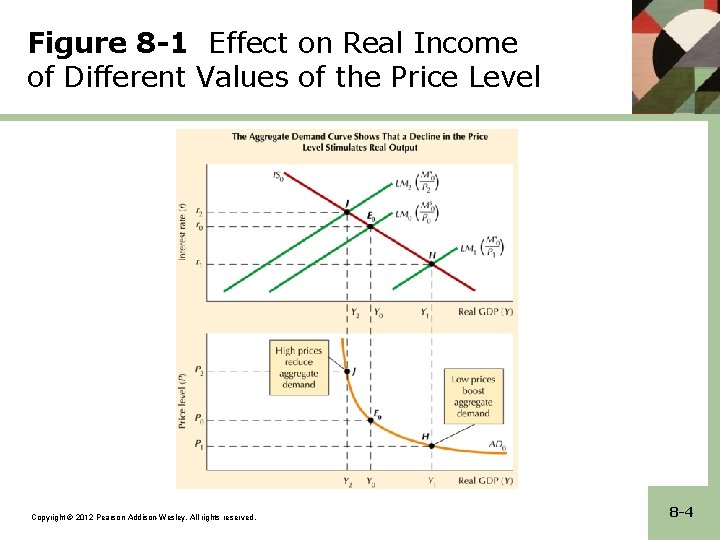
Aggregate Demand • The aggregate demand (AD) curve shows the different combinations of the price level and real output at which the money and commodity markets are both in equilibrium • Recall: Any increase in C + I + G + NX will cause the AD curve to shift to the right Copyright © 2012 Pearson Addison-Wesley. All rights reserved. 8 -3

Figure 8 -1 Effect on Real Income of Different Values of the Price Level Copyright © 2012 Pearson Addison-Wesley. All rights reserved. 8 -4

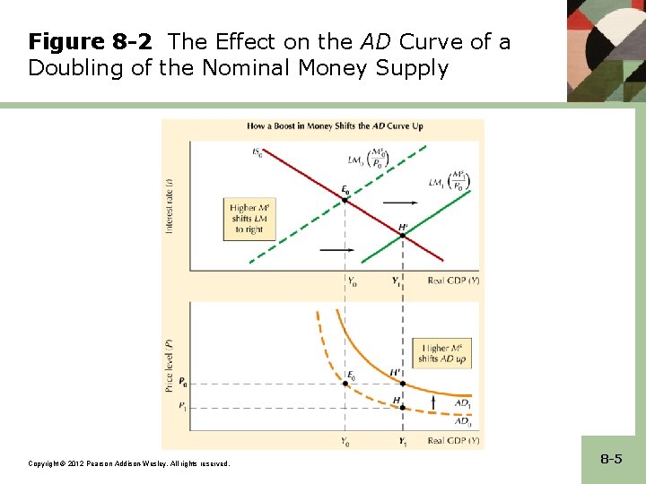
Figure 8 -2 The Effect on the AD Curve of a Doubling of the Nominal Money Supply Copyright © 2012 Pearson Addison-Wesley. All rights reserved. 8 -5

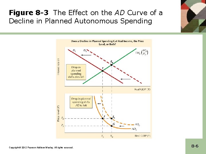
Figure 8 -3 The Effect on the AD Curve of a Decline in Planned Autonomous Spending Copyright © 2012 Pearson Addison-Wesley. All rights reserved. 8 -6

AD and the Global Economic Crisis • The global economic crisis starting in 2008 occurred primarily because of a sharp leftward shift in AD – Crisis originated in the U. S. financial market due to the bursting of the housing bubble caused by: • • Lax regulation Financial innovation Securitization Highly stimulative monetary policy – Spread to foreign countries via interconnected capital markets and foreign ownership of “toxic” MBS’s • Aggregate supply (see next slide) did not play an important role because the inflation rate and price level remained stable Copyright © 2012 Pearson Addison-Wesley. All rights reserved. 8 -7

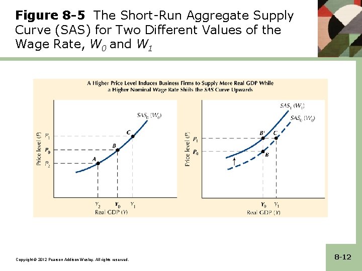
Aggregate Supply • The Short-Run Aggregate Supply (SAS) curve shows the amount of output that business firms are willing to produce at different price levels, holding constant the nominal wage rate – The SAS curve is upward sloping since an increase in the price level will increase profits for firms assuming wages and other input costs are fixed. This results in firms increasing output at higher prices • The Long-Run Aggregate Supply (LAS) curve shows the amount that business firms are willing to produce when the nominal wage rate has fully adjusted to any changes in the price level Copyright © 2012 Pearson Addison-Wesley. All rights reserved. 8 -8

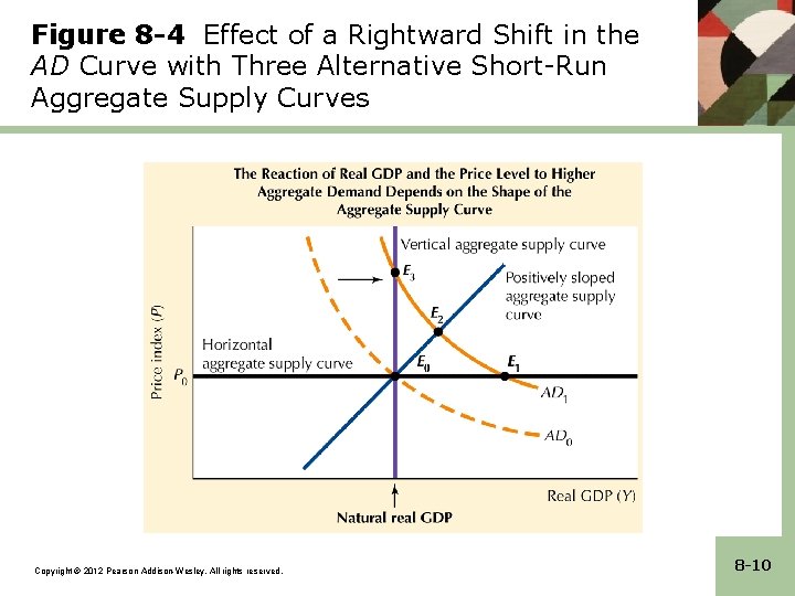
Controversies Surrounding AS • The three possible shapes of the AS curve has created decades of controversy. • The horizontal AS curve assumes prices are fixed, but is unrealistic because it cannot explain inflation. • The vertical AS curve assumes prices are perfectly flexible and is useful to analyze inflation, but cannot explain unemployment. • The positively sloped short run AS curve assumes that wages are fixed, so it cannot be applied to the long run, but it helps to explain short -run fluctuations in output. Copyright © 2012 Pearson Addison-Wesley. All rights reserved. 8 -9

Figure 8 -4 Effect of a Rightward Shift in the AD Curve with Three Alternative Short-Run Aggregate Supply Curves Copyright © 2012 Pearson Addison-Wesley. All rights reserved. 8 -10

Deriving the SAS Curve • Assume that wages are fixed in the short run and that prices are merely “sticky. ” • If prices rise, firms benefit because the real wage paid to their workers falls. • Thus, firms can increase output if the price level rises because their profits increase! – P but W fixed Y SAS curve is upward sloping! Copyright © 2012 Pearson Addison-Wesley. All rights reserved. 8 -11

Figure 8 -5 The Short-Run Aggregate Supply Curve (SAS) for Two Different Values of the Wage Rate, W 0 and W 1 Copyright © 2012 Pearson Addison-Wesley. All rights reserved. 8 -12

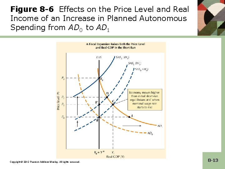
Figure 8 -6 Effects on the Price Level and Real Income of an Increase in Planned Autonomous Spending from AD 0 to AD 1 Copyright © 2012 Pearson Addison-Wesley. All rights reserved. 8 -13

Interpretations of the Business Cycle • The theory discussed in Figure 8 -6 assumes that prices are flexible while wages are fixed – This implies a countercyclical movement in the real wage: Y↑ (W/P)↓ – But statistical evidence do not show consistent or strong countercyclical real wages • An alternative view is that both prices and wages are sticky in the short run SAS relatively flat – When GDP rises above natural real GDP, there is inflationary pressure that causes both W and P to rise – Wage and price rigidity theories discussed in Ch 17 Copyright © 2012 Pearson Addison-Wesley. All rights reserved. 8 -14

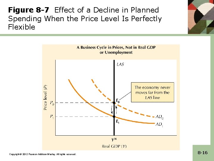
The Quantity Theory of Money • Classical economists believed that flexible prices were the self-correcting forces that could stabilize real GDP – Believed that U was voluntary and/or transitory condition – Alfred Pigou (1913) argued that U came from the slow adjustment of wages that kept labor markets from equilibrium • The “Quantity Equation” was a model developed by classical economists: MSV = PY • The Quantity Theory of Money holds that: – Actual output tends to grow steadily – Velocity is determined by payment practices – MS changes therefore affect the price level and have little effect on output Copyright © 2012 Pearson Addison-Wesley. All rights reserved. 8 -15

Figure 8 -7 Effect of a Decline in Planned Spending When the Price Level Is Perfectly Flexible Copyright © 2012 Pearson Addison-Wesley. All rights reserved. 8 -16

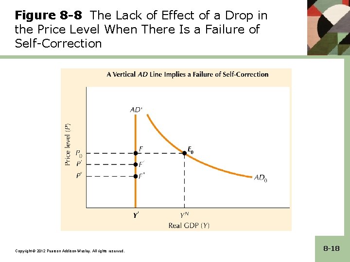
The Failure of Self-Correction • The Keynesian Revolution started with publication of John Maynard Keyne’s The General Theory in 1936 in response to failures of classical economic ideas during The Great Depression. • Monetary Impotence is the failure of real GDP to respond to an increase in the real MS when: – The IS curve is vertical – The LM curve is horizontal (i. e. Liquidity Trap) – “Zero lower bound” is reached: r ≥ 0 • Rigid Wages refers to the failure of the nominal wage rate to adjust by the amount needed to maintain equilibrium in the labor market. Copyright © 2012 Pearson Addison-Wesley. All rights reserved. 8 -17

Figure 8 -8 The Lack of Effect of a Drop in the Price Level When There Is a Failure of Self-Correction Copyright © 2012 Pearson Addison-Wesley. All rights reserved. 8 -18

Stabilizing and Destabilizing Effects of P • Stabilizing Effects of P – The Pigou or Real Balance Effect is the direct stimulus to AD caused by an increase in the real money supply and does not require a decline in the interest rate. – The Keynes Effect is the stimulus to AD caused by a decline in the interest rate. • Destabilizing Effects of P – The Expectations Effect is the decline in AD caused by the postponement of purchases when consumers expect P. – The Redistribution Effect is the decline in AD caused by the effect of falling prices in redistributing income from high-spending debtors to low-spending savers. Copyright © 2012 Pearson Addison-Wesley. All rights reserved. 8 -19

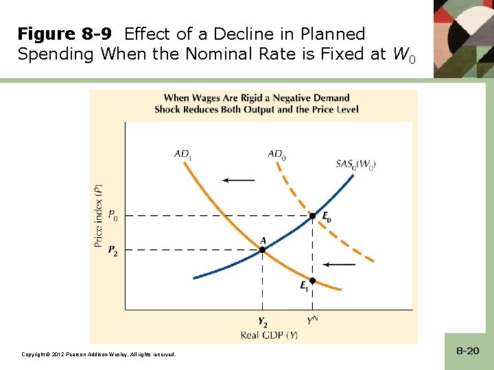
Figure 8 -9 Effect of a Decline in Planned Spending When the Nominal Rate is Fixed at W 0 Copyright © 2012 Pearson Addison-Wesley. All rights reserved. 8 -20

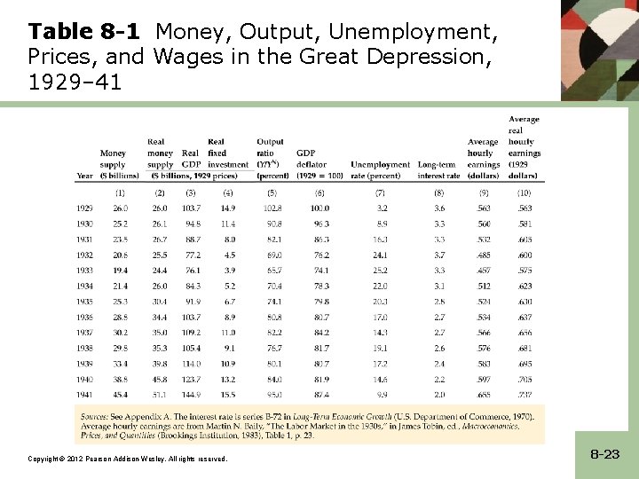
What Caused the Great Depression? • Real investment fell by 74% from 1929 to 1933 • Sharp fall in consumption spending • Fall in NX due to failure to devalue the USD until 1933 and protective tariffs • Bank failures • Tight monetary policy: nominal MS fell by 25% from 1929 to 1933 • No price decline from 1936 to 1940 – 26% decline from 1929 to 1933 Copyright © 2012 Pearson Addison-Wesley. All rights reserved. 8 -21

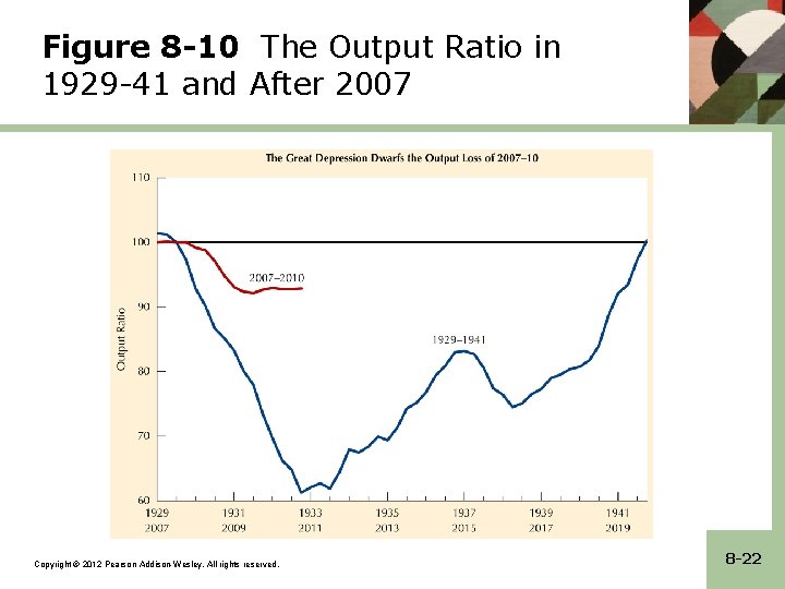
Figure 8 -10 The Output Ratio in 1929 -41 and After 2007 Copyright © 2012 Pearson Addison-Wesley. All rights reserved. 8 -22

Table 8 -1 Money, Output, Unemployment, Prices, and Wages in the Great Depression, 1929– 41 Copyright © 2012 Pearson Addison-Wesley. All rights reserved. 8 -23

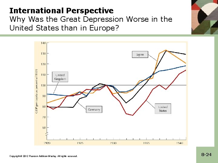
International Perspective Why Was the Great Depression Worse in the United States than in Europe? Copyright © 2012 Pearson Addison-Wesley. All rights reserved. 8 -24

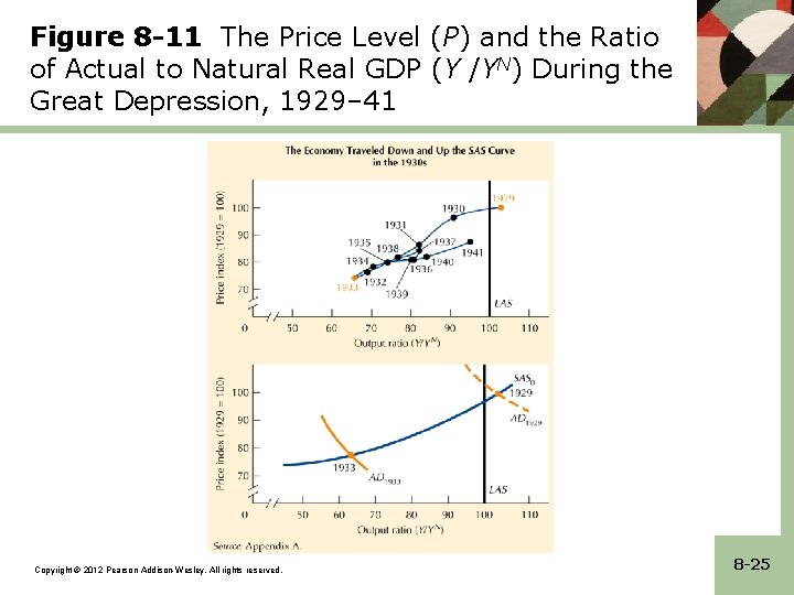
Figure 8 -11 The Price Level (P) and the Ratio of Actual to Natural Real GDP (Y /YN) During the Great Depression, 1929– 41 Copyright © 2012 Pearson Addison-Wesley. All rights reserved. 8 -25