Chapter 7 The Query Compiler Query Processor Query

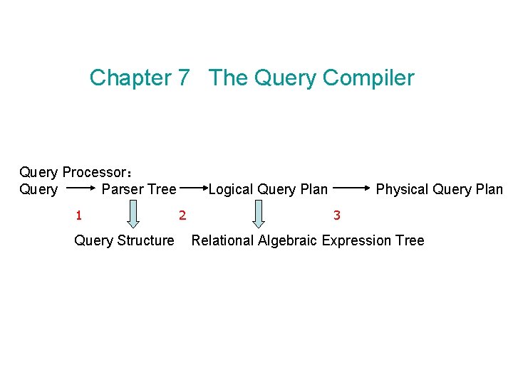
Chapter 7 The Query Compiler Query Processor： Query Parser Tree 1 Query Structure Logical Query Plan 2 Physical Query Plan 3 Relational Algebraic Expression Tree

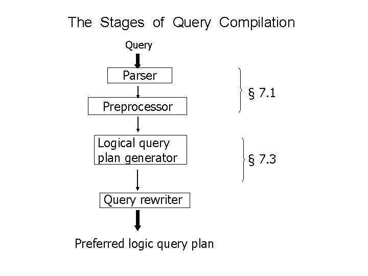
The Stages of Query Compilation Query Parser Preprocessor Logical query plan generator Query rewriter Preferred logic query plan § 7. 1 § 7. 3

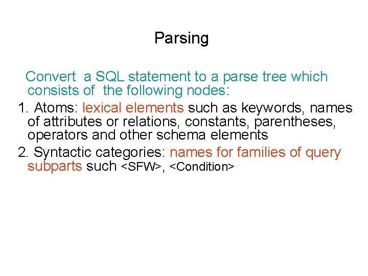
Parsing Convert a SQL statement to a parse tree which consists of the following nodes: 1. Atoms: lexical elements such as keywords, names of attributes or relations, constants, parentheses, operators and other schema elements 2. Syntactic categories: names for families of query subparts such <SFW>, <Condition>

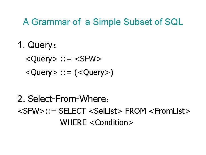
A Grammar of a Simple Subset of SQL 1. Query： <Query> : : = <SFW> <Query> : : = (<Query>) 2. Select-From-Where： <SFW>: : = SELECT <Sel. List> FROM <From. List> WHERE <Condition>

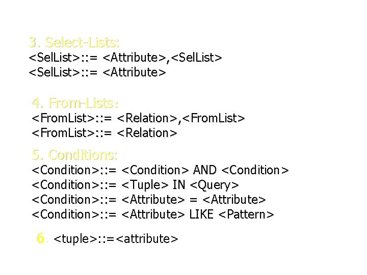
3. Select-Lists: <Sel. List>: : = <Attribute>, <Sel. List>: : = <Attribute> 4. From-Lists： <From. List>: : = <Relation>, <From. List>: : = <Relation> 5. Conditions: <Condition>: : = <Condition> AND <Condition>: : = <Tuple> IN <Query> <Condition>: : = <Attribute> LIKE <Pattern> 6. <tuple>: : =<attribute>

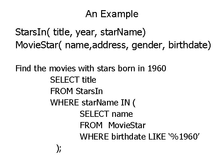
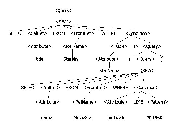
An Example Stars. In( title, year, star. Name) Movie. Star( name, address, gender, birthdate) Find the movies with stars born in 1960 SELECT title FROM Stars. In WHERE star. Name IN ( SELECT name FROM Movie. Star WHERE birthdate LIKE ‘%1960’ );

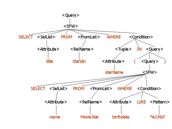
<Query> <SFW> SELECT <Sel. List> FROM <Attribute> title <From. List> WHERE <Rel. Name> Stars. In <Condition> <Tuple> <Attribute> star. Name SELECT <Sel. List> FROM <From. List> WHERE <Attribute> <Rel. Name> <Attribute> name Movie. Star birthdate IN <Query> ( <Query> ) <SFW> <Condition> LIKE <Pattern> ‘%1960’

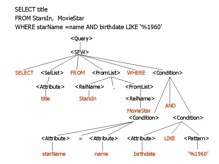
SELECT title FROM Stars. In, Movie. Star WHERE star. Name =name AND birthdate LIKE ‘%1960’ <Query> <SFW> SELECT <Sel. List> <Attribute> title FROM <From. List> <Rel. Name> , Stars. In WHERE <Condition> <From. List> <Rel. Name> Movie. Star <Condition> <Attribute> star. Name = <Attribute> name <Attribute> birthdate AND <Condition> LIKE <Pattern> ‘%1960’

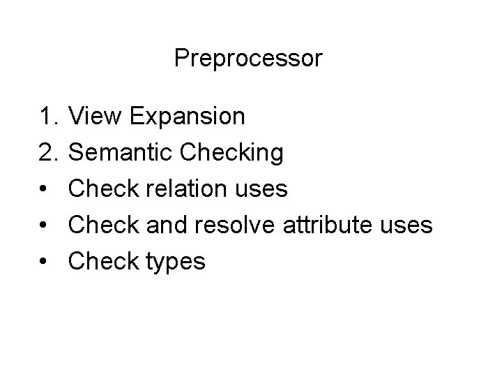
　Preprocessor 1. 2. • • • View Expansion Semantic Checking Check relation uses Check and resolve attribute uses Check types

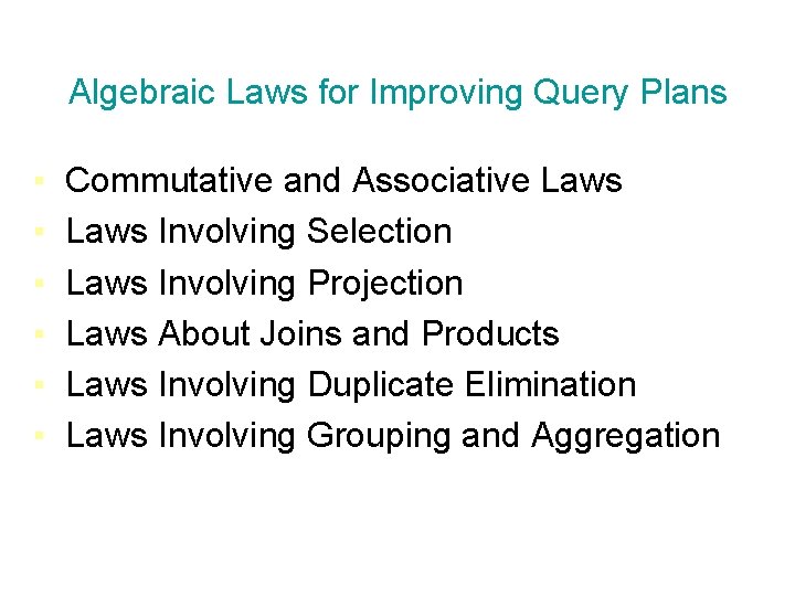
Algebraic Laws for Improving Query Plans ▪ ▪ ▪ Commutative and Associative Laws Involving Selection Laws Involving Projection Laws About Joins and Products Laws Involving Duplicate Elimination Laws Involving Grouping and Aggregation

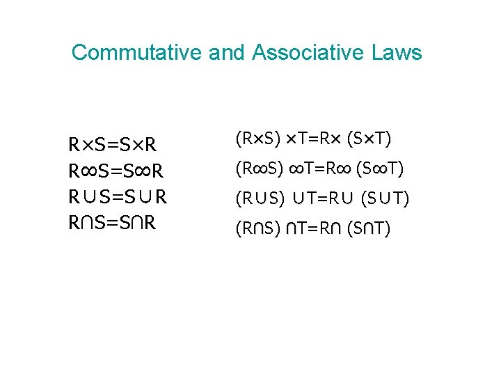
Commutative and Associative Laws R×S=S×R R∞S=S∞R R∪S=S∪R R∩S=S∩R (R×S) ×T=R× (S×T) (R∞S) ∞T=R∞ (S∞T) (R∪S) ∪T=R∪ (S∪T) (R∩S) ∩T=R∩ (S∩T)

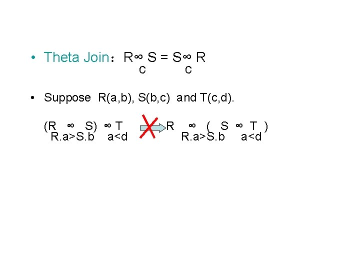
• Theta Join：R∞ S = S∞ R c c • Suppose R(a, b), S(b, c) and T(c, d). (R ∞ S) ∞ T R. a>S. b a<d R ∞ ( S ∞ T ) R. a>S. b a<d

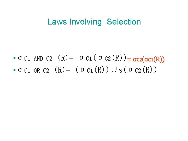
Laws Involving Selection ▪σC 1 AND C 2 OR C 2 (R)= σC 1(σC 2(R))= σC 2(σC 1(R)) (R)= (σC 1(R))∪s(σC 2(R))

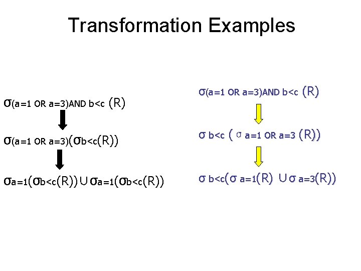
Transformation Examples σ(a=1 OR a=3)AND b<c (R) σ(a=1 OR a=3)(σb<c(R)) σ b<c (σa=1 OR a=3 (R)) σa=1(σb<c(R))∪σa=1(σb<c(R)) σ b<c(σ a=1(R) ∪σ a=3(R))

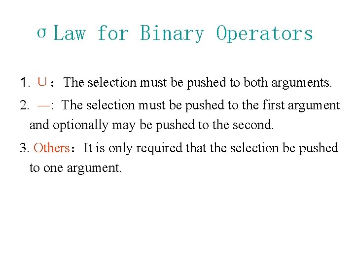
σLaw for Binary Operators 1. ∪：The selection must be pushed to both arguments. 2. ―: The selection must be pushed to the first argument and optionally may be pushed to the second. 3. Others：It is only required that the selection be pushed to one argument.

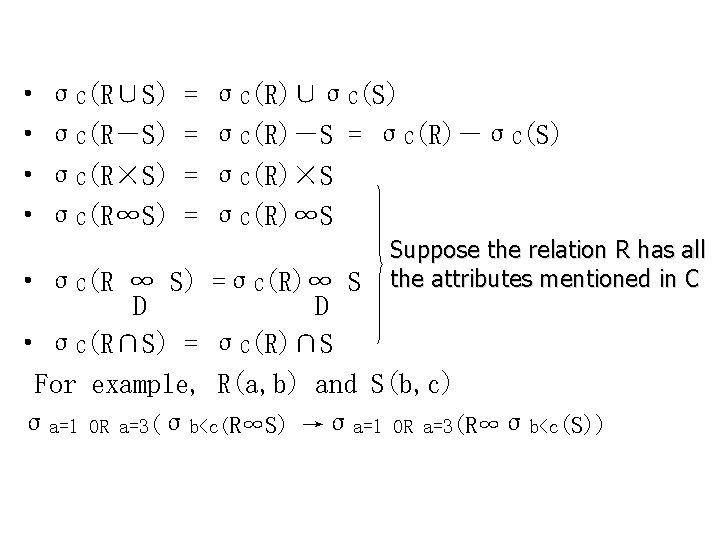
• • σC(R∪S) σC(R―S) σC(R×S) σC(R∞S) = = σC(R)∪σC(S) σC(R)―S = σC(R)―σC(S) σC(R)×S σC(R)∞S Suppose the relation R has all the attributes mentioned in C • σC(R ∞ S) =σC(R)∞ S D D • σC(R∩S) = σC(R)∩S For example, R(a, b) and S(b, c) σa=1 OR a=3(σb<c(R∞S) →σa=1 OR a=3(R∞σb<c(S))

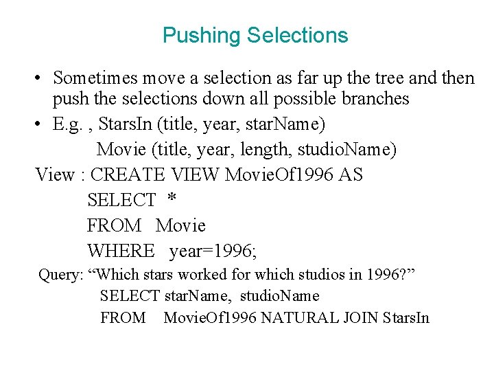
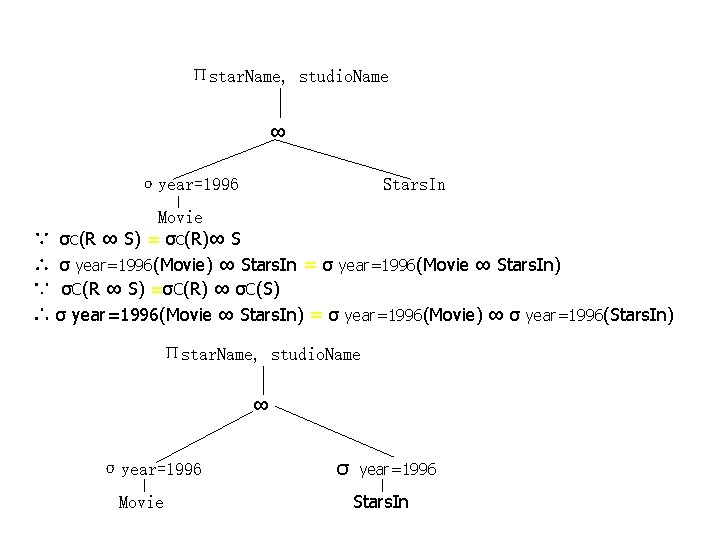
Pushing Selections • Sometimes move a selection as far up the tree and then push the selections down all possible branches • E. g. , Stars. In (title, year, star. Name) Movie (title, year, length, studio. Name) View : CREATE VIEW Movie. Of 1996 AS SELECT * FROM Movie WHERE year=1996; Query: “Which stars worked for which studios in 1996? ” SELECT star. Name, studio. Name FROM Movie. Of 1996 NATURAL JOIN Stars. In

Пstar. Name, studio. Name ∞ σyear=1996 ∵ ∴ Stars. In Movie σC(R ∞ S) = σC(R)∞ S σ year=1996(Movie) ∞ Stars. In = σ year=1996(Movie ∞ Stars. In) σC(R ∞ S) =σC(R) ∞ σC(S) σ year=1996(Movie ∞ Stars. In) = σ year=1996(Movie) ∞ σ year=1996(Stars. In) Пstar. Name, studio. Name ∞ σyear=1996 Movie σ year=1996 Stars. In

Laws Involving Projection A projection may be introduced anywhere in an expression tree, as long as it eliminates only attributes that are never used by any of the operators above, and are not in the result of the entire expression.

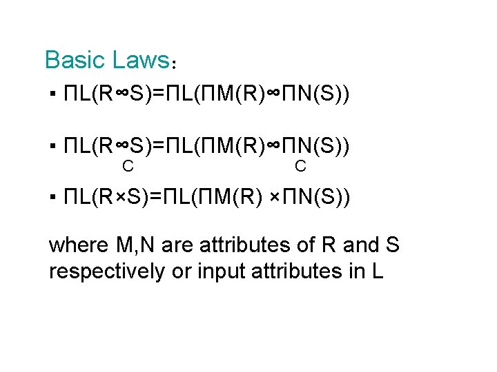
Basic Laws： ▪ ПL(R∞S)=ПL(ПM(R)∞ПN(S)) C C ▪ ПL(R×S)=ПL(ПM(R) ×ПN(S)) where M, N are attributes of R and S respectively or input attributes in L

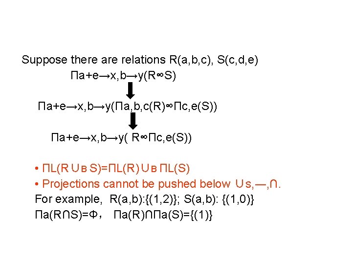
Suppose there are relations R(a, b, c), S(c, d, e) Пa+e→x, b→y(R∞S) Пa+e→x, b→y(Пa, b, c(R)∞Пc, e(S)) Пa+e→x, b→y( R∞Пc, e(S)) • ПL(R∪B S)=ПL(R)∪B ПL(S) • Projections cannot be pushed below ∪S, ―, ∩. For example, R(a, b): {(1, 2)}; S(a, b): {(1, 0)} Пa(R∩S)=Φ， Пa(R)∩Пa(S)={(1)}

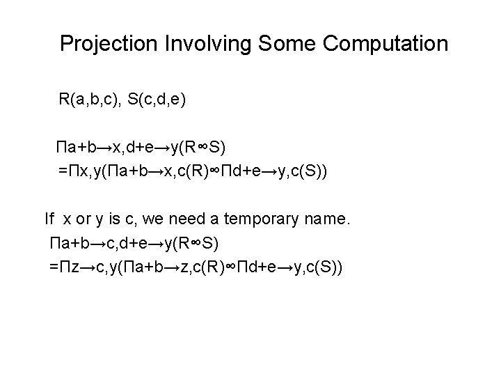
Projection Involving Some Computation R(a, b, c), S(c, d, e) Пa+b→x, d+e→y(R∞S) =Пx, y(Пa+b→x, c(R)∞Пd+e→y, c(S)) If x or y is c, we need a temporary name. Пa+b→c, d+e→y(R∞S) =Пz→c, y(Пa+b→z, c(R)∞Пd+e→y, c(S))

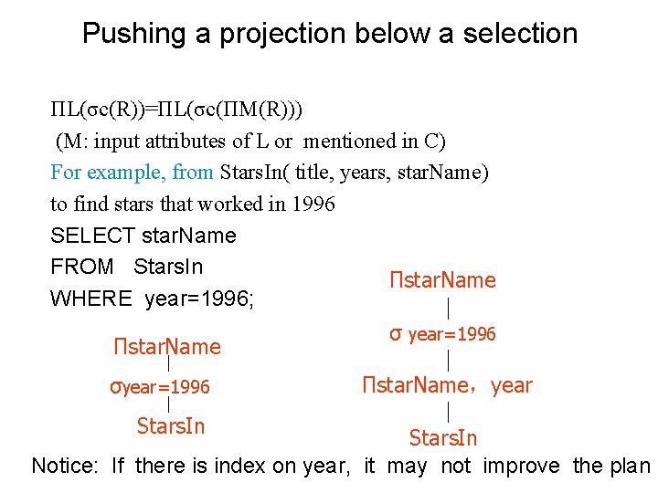
Pushing a projection below a selection ПL(σc(R))=ПL(σc(ПM(R))) (M: input attributes of L or mentioned in C) For example, from Stars. In( title, years, star. Name) to find stars that worked in 1996 SELECT star. Name FROM Stars. In Пstar. Name WHERE year=1996; Пstar. Name σyear=1996 Stars. In σ year=1996 Пstar. Name，year Stars. In Notice: If there is index on year, it may not improve the plan

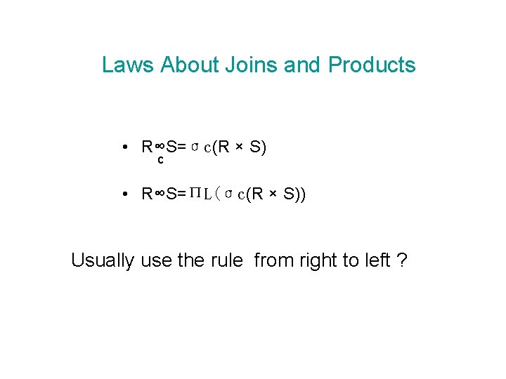
Laws About Joins and Products • R∞S=σc(R × S) c • R∞S=ПL(σc(R × S)) Usually use the rule from right to left ?

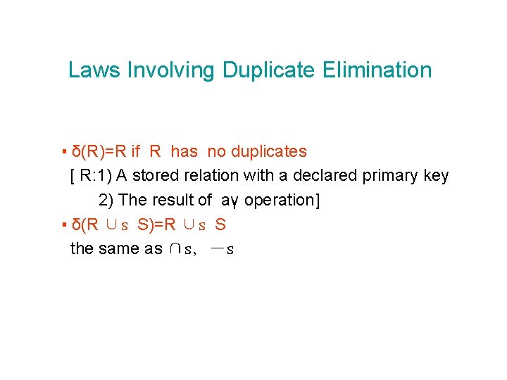
Laws Involving Duplicate Elimination ▪ δ(R)=R if R has no duplicates [ R: 1) A stored relation with a declared primary key 2) The result of aγ operation] ▪ δ(R ∪s S)=R ∪s S the same as ∩s, ―s

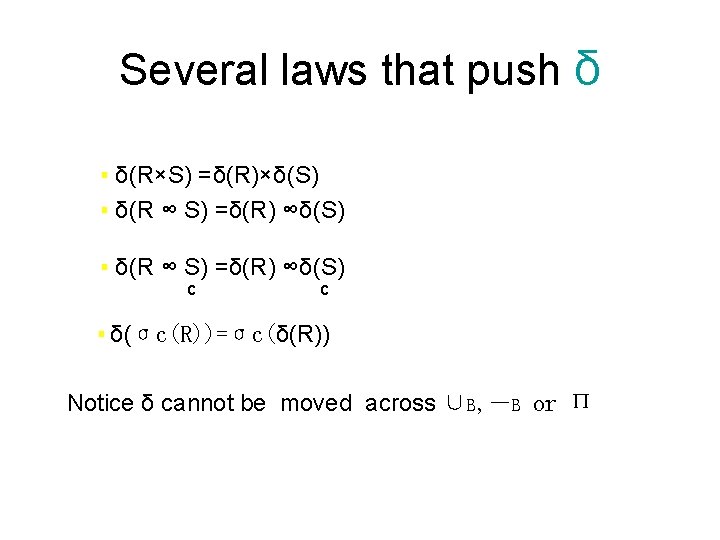
Several laws that push δ ▪ δ(R×S) =δ(R)×δ(S) ▪ δ(R ∞ S) =δ(R) ∞δ(S) c c ▪ δ(σc(R))=σc(δ(R)) Notice δ cannot be moved across ∪B, ―B or П

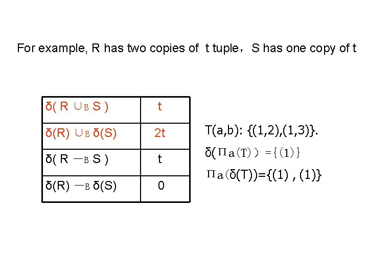
For example, R has two copies of t tuple，S has one copy of t δ( R ∪B S ) t δ(R) ∪B δ(S) 2 t δ( R ―B S ) t δ(R) ―B δ(S) 0 T(a, b): {(1, 2), (1, 3)}. δ(Пa(T)）={(1)} Пa(δ(T))={(1) , (1)}

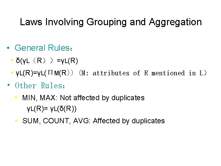
Laws Involving Grouping and Aggregation • General Rules： ▪ δ(γL（R））=γL(R) ▪ γL(R)=γL(ПM(R)) (M: attributes of R mentioned in L） • Other Rules： ▪ MIN, MAX: Not affected by duplicates γL(R)= γL(δ(R)) ▪ SUM, COUNT, AVG: Affected by duplicates

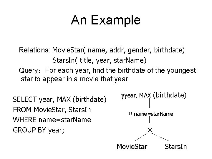
An Example Relations: Movie. Star( name, addr, gender, birthdate) Stars. In( title, year, star. Name) Query：For each year, find the birthdate of the youngest star to appear in a movie that year SELECT year, MAX (birthdate) FROM Movie. Star, Stars. In WHERE name=star. Name GROUP BY year; γyear, MAX (birthdate) σname=star. Name × Movie. Stars. In

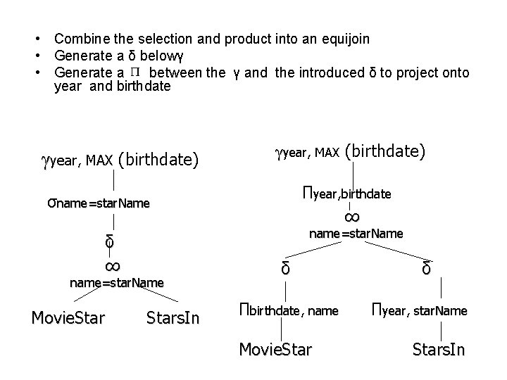
• Combine the selection and product into an equijoin • Generate a δ belowγ • Generate a П between the γ and the introduced δ to project onto year and birthdate γyear, MAX (birthdate) Пyear, birthdate ∞ σname=star. Name δ ∞ name=star. Name Movie. Stars. In δ Пbirthdate, name Movie. Star δ Пyear, star. Name Stars. In

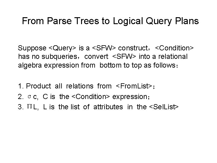
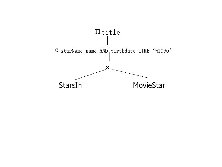
From Parse Trees to Logical Query Plans Suppose <Query> is a <SFW> construct，<Condition> has no subqueries，convert <SFW> into a relational algebra expression from bottom to top as follows： 1. Product all relations from <From. List>； 2. σc, C is the <Condition> expression； 3. ПL, L is the list of attributes in the <Sel. List>

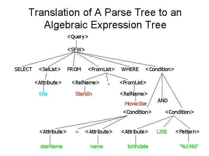
Translation of A Parse Tree to an Algebraic Expression Tree <Query> <SFW> SELECT <Sel. List> <Attribute> title FROM <From. List> <Rel. Name> , Stars. In WHERE <Condition> <From. List> <Rel. Name> Movie. Star <Condition> <Attribute> star. Name = <Attribute> name <Attribute> birthdate AND <Condition> LIKE <Pattern> ‘%1960’

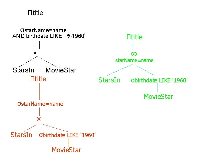
Пtitle σstar. Name=name AND birthdate LIKE‘%1960’ × Stars. In Movie. Star

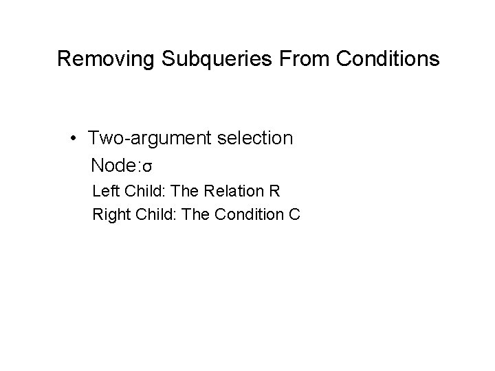
Removing Subqueries From Conditions • Two-argument selection Node: σ Left Child: The Relation R Right Child: The Condition C

<Query> <SFW> SELECT <Sel. List> FROM <Attribute> title <From. List> WHERE <Rel. Name> Stars. In <Condition> <Tuple> <Attribute> star. Name SELECT <Sel. List> FROM <From. List> WHERE <Attribute> <Rel. Name> <Attribute> name Movie. Star birthdate IN <Query> ( <Query> ) <SFW> <Condition> LIKE <Pattern> ‘%1960’

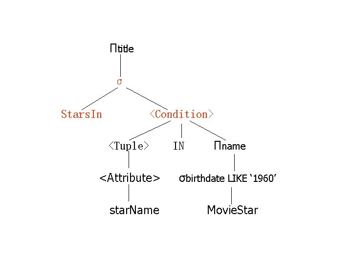
Пtitle σ Stars. In <Condition> <Tuple> <Attribute> star. Name IN Пname σbirthdate LIKE ‘ 1960’ Movie. Star

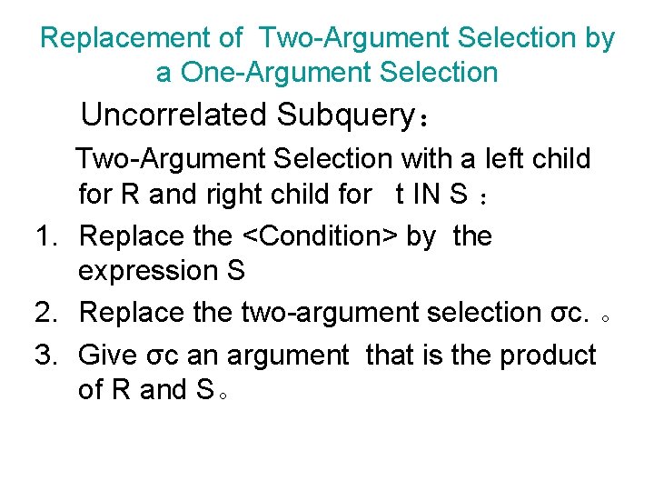
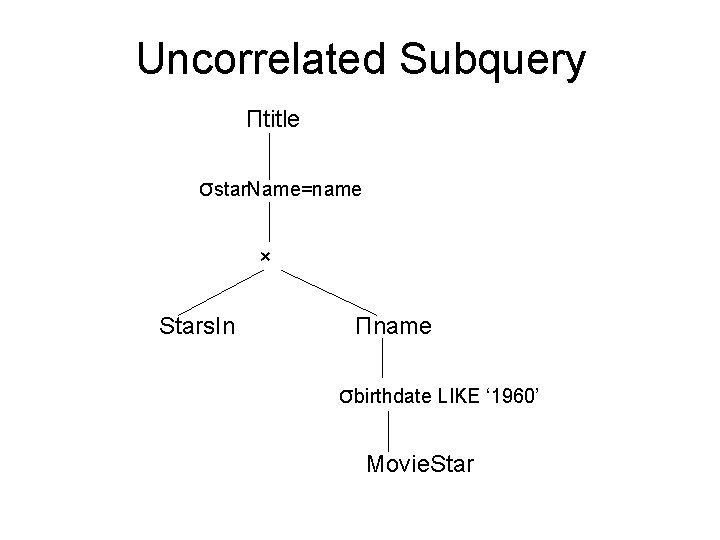
Replacement of Two-Argument Selection by a One-Argument Selection Uncorrelated Subquery： Two-Argument Selection with a left child for R and right child for t IN S ： 1. Replace the <Condition> by the expression S 2. Replace the two-argument selection σc. 。 3. Give σc an argument that is the product of R and S。

Uncorrelated Subquery Пtitle σstar. Name=name × Stars. In Пname σbirthdate LIKE ‘ 1960’ Movie. Star

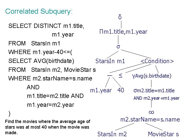
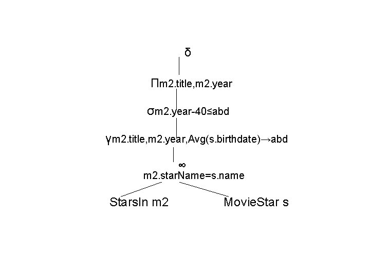
Correlated Subquery: δ SELECT DISTINCT m 1. title, Пm 1. title, m 1. year FROM Stars. In m 1 σ WHERE m 1. year-40<=( SELECT AVG(birthdate) Stars. In m 1 <Condition> FROM Stars. In m 2, Movie. Star s ― ≤ γAvg(s. birthdate) WHERE m 2. star. Name=s. name AND m 1. year 40 σm 2. title=m 1. title=m 2. title AND m 2. year=m 1. year=m 2. year ∞ ) m 2. star. Name=s. name Find the movies where the average of stars was at most 40 when the movie was made. Stars. In m 2 Movie. Star s

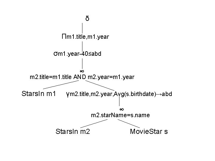
δ Пm 1. title, m 1. year σm 1. year-40≤abd ∞ m 2. title=m 1. title AND m 2. year=m 1. year Stars. In m 1 γm 2. title, m 2. year, Avg(s. birthdate)→abd ∞ m 2. star. Name=s. name Stars. In m 2 Movie. Star s

δ Пm 2. title, m 2. year σm 2. year-40≤abd γm 2. title, m 2. year, Avg(s. birthdate)→abd ∞ m 2. star. Name=s. name Stars. In m 2 Movie. Star s

Improving the Logical Query Plan • Pushing down selection. • Pushing down projection，or adding new projection. • Removing duplicate elimination, or moving to a more convenient position. • Turning selection and product into an equijoin.

Пtitle σstar. Name=name AND birthdate LIKE ‘%1960’ Пtitle ∞ × star. Name=name Stars. In Movie. Star Пtitle σstar. Name=name × Stars. In σbirthdate LIKE ‘ 1960’ Movie. Star

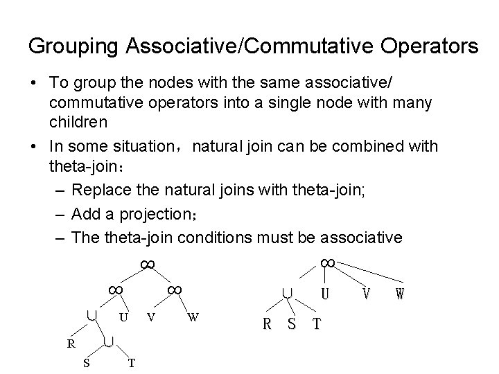
Grouping Associative/Commutative Operators • To group the nodes with the same associative/ commutative operators into a single node with many children • In some situation，natural join can be combined with theta-join： – Replace the natural joins with theta-join; – Add a projection； – The theta-join conditions must be associative ∞ ∞ ∞ ∪ ∞ U ∪ R S T V ∪ W U R S T V W

Estimating the Cost of Operations When deriving physical plans from a logical plan, we need select 1. 2. 3. 4. an order and grouping for associative-and-commutative operations； an algorithm for each operator in the logical plan； additional operators – scanning, sorting, and so on； the way in which arguments are passed from one operator to the next

Estimating Sizes of Intermediate Relations • • • Give accurate estimates Are easy to compute Are logically consistent

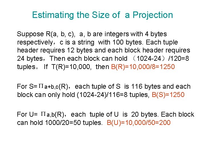
Estimating the Size of a Projection Suppose R(a, b, c), a, b are integers with 4 bytes respectively，c is a string with 100 bytes. Each tuple header requires 12 bytes and each block header requires 24 bytes，Then each block can hold （1024 -24）/120=8 tuples。 If T(R)=10, 000, then B(R)=10, 000/8=1250 For S=Пa+b, c(R)，each tuple of S is 116 bytes and each block can only hold (1024 -24)/116=8 tuples, B(S)=1250 For U= Пa, b(R)，each tuple of U is 20 bytes. Each block can hold 1000/20=50 tuples. B(U)=10, 000/50=200

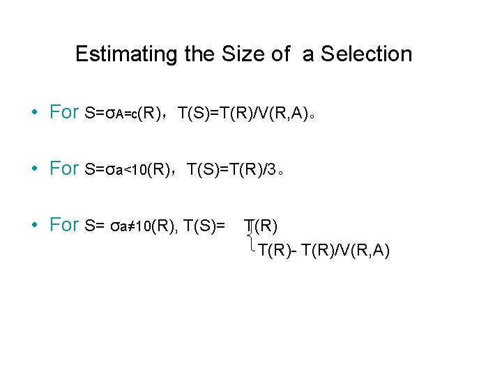
Estimating the Size of a Selection • For S=σA=c(R)，T(S)=T(R)/V(R, A)。 • For S=σa<10(R)，T(S)=T(R)/3。 • For S= σa≠ 10(R), T(S)= T(R)- T(R)/V(R, A)

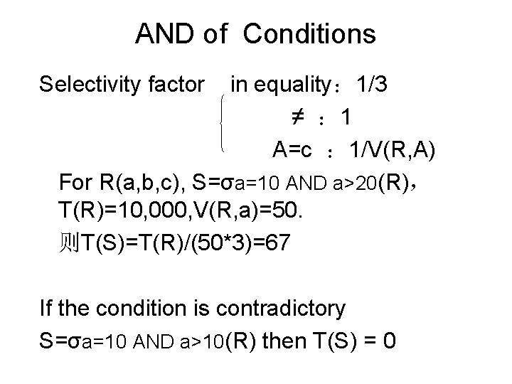
AND of Conditions Selectivity factor in equality： 1/3 ≠ ： 1 A=c ： 1/V(R, A) For R(a, b, c), S=σa=10 AND a>20(R)， T(R)=10, 000, V(R, a)=50. 则T(S)=T(R)/(50*3)=67 If the condition is contradictory S=σa=10 AND a>10(R) then T(S) = 0

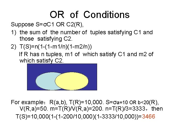
OR of Conditions Suppose S=σC 1 OR C 2(R), 1) the sum of the number of tuples satisfying C 1 and those satisfying C 2. 2) T(S)=n(1 -(1 -m 1/n)(1 -m 2/n)) If R has n tuples, m 1 of which satisfy C 1 and m 2 of which satisfy C 2. For example：R(a, b), T(R)=10, 000. S=σa=10 OR b<20(R), V(R, a)=50. m=T(R)/V(R, a)=200. n=T(R)/3=3333，then T(S)=10, 000(1 -(1 -200/10, 000)(1 -3333/10, 000))=3466

Estimating the Size of a Join 1. The equijoin can be handled as the natural join； 2. The theta-join can be handled as a selection following a product.

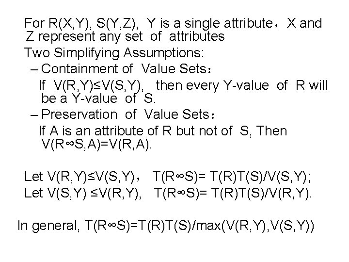
For R(X, Y), S(Y, Z), Y is a single attribute，X and Z represent any set of attributes Two Simplifying Assumptions: – Containment of Value Sets： If V(R, Y)≤V(S, Y), then every Y-value of R will be a Y-value of S. – Preservation of Value Sets： If A is an attribute of R but not of S, Then V(R∞S, A)=V(R, A). Let V(R, Y)≤V(S, Y)， T(R∞S)= T(R)T(S)/V(S, Y); Let V(S, Y) ≤V(R, Y), T(R∞S)= T(R)T(S)/V(R, Y). In general, T(R∞S)=T(R)T(S)/max(V(R, Y), V(S, Y))

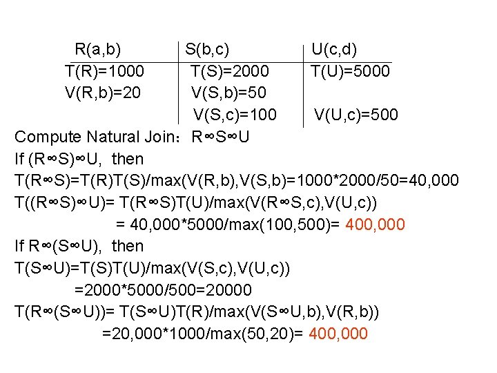
R(a, b) T(R)=1000 V(R, b)=20 S(b, c) U(c, d) T(S)=2000 T(U)=5000 V(S, b)=50 V(S, c)=100 V(U, c)=500 Compute Natural Join：R∞S∞U If (R∞S)∞U, then T(R∞S)=T(R)T(S)/max(V(R, b), V(S, b)=1000*2000/50=40, 000 T((R∞S)∞U)= T(R∞S)T(U)/max(V(R∞S, c), V(U, c)) = 40, 000*5000/max(100, 500)= 400, 000 If R∞(S∞U), then T(S∞U)=T(S)T(U)/max(V(S, c), V(U, c)) =2000*5000/500=20000 T(R∞(S∞U))= T(S∞U)T(R)/max(V(S∞U, b), V(R, b)) =20, 000*1000/max(50, 20)= 400, 000

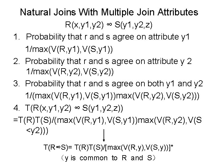
Natural Joins With Multiple Join Attributes R(x, y 1, y 2) ∞ S(y 1, y 2, z) 1. Probability that r and s agree on attribute y 1 1/max(V(R, y 1), V(S, y 1)) 2. Probability that r and s agree on attribute y 2 1/max(V(R, y 2), V(S, y 2)) 3. Probability that r and s agree on both y 1 and y 2 1/(max(V(R, y 1), V(S, y 1))max(V(R, y 2), V(S, y 2))) 4. T(R(x, y 1, y 2) ∞ S(y 1, y 2, z)) =T(R)T(S)/(max(V(R, y 1), V(S, y 1))max(V(R, y 2), V(S <y 2))) T(R∞S)= T(R)T(S)/[max(V(R, y), V(S, y))]* （y is common to R and S）

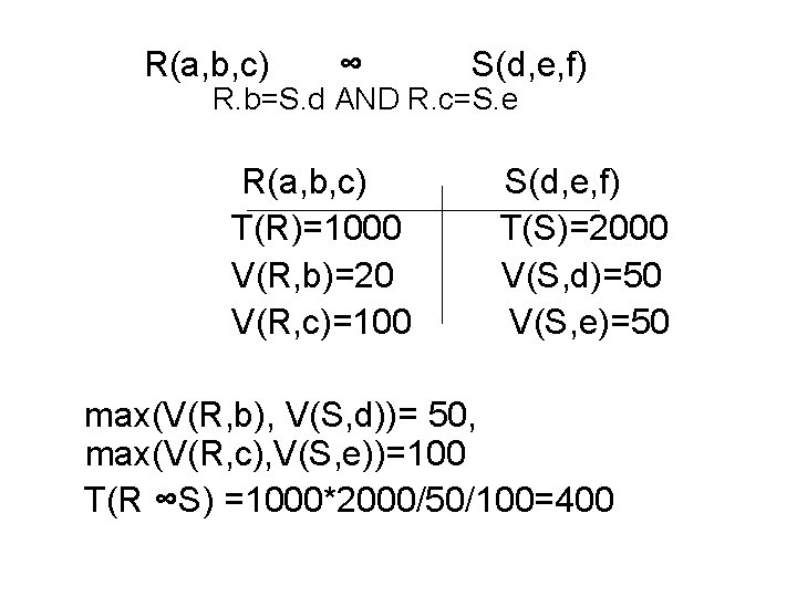
R(a, b, c) ∞ S(d, e, f) R. b=S. d AND R. c=S. e R(a, b, c) T(R)=1000 V(R, b)=20 V(R, c)=100 S(d, e, f) T(S)=2000 V(S, d)=50 V(S, e)=50 max(V(R, b), V(S, d))= 50, max(V(R, c), V(S, e))=100 T(R ∞S) =1000*2000/50/100=400

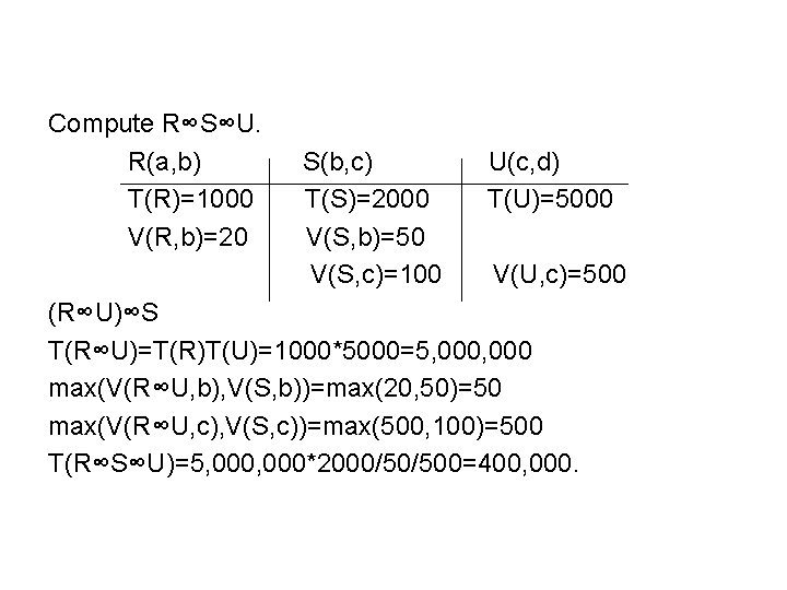
Compute R∞S∞U. R(a, b) T(R)=1000 V(R, b)=20 S(b, c) T(S)=2000 V(S, b)=50 V(S, c)=100 U(c, d) T(U)=5000 V(U, c)=500 (R∞U)∞S T(R∞U)=T(R)T(U)=1000*5000=5, 000 max(V(R∞U, b), V(S, b))=max(20, 50)=50 max(V(R∞U, c), V(S, c))=max(500, 100)=500 T(R∞S∞U)=5, 000*2000/50/500=400, 000.

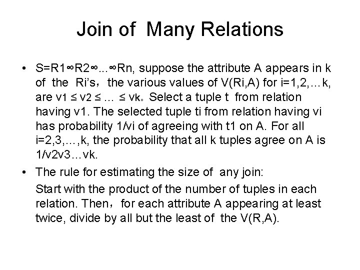
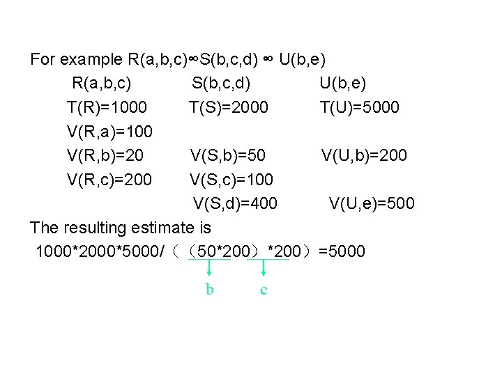
Join of Many Relations • S=R 1∞R 2∞. . . ∞Rn, suppose the attribute A appears in k of the Ri’s，the various values of V(Ri, A) for i=1, 2, …k, are v 1 ≤ v 2 ≤ … ≤ vk。Select a tuple t from relation having v 1. The selected tuple ti from relation having vi has probability 1/vi of agreeing with t 1 on A. For all i=2, 3, …, k, the probability that all k tuples agree on A is 1/v 2 v 3…vk. • The rule for estimating the size of any join: Start with the product of the number of tuples in each relation. Then，for each attribute A appearing at least twice, divide by all but the least of the V(R, A).

For example R(a, b, c)∞S(b, c, d) ∞ U(b, e) R(a, b, c) S(b, c, d) U(b, e) T(R)=1000 T(S)=2000 T(U)=5000 V(R, a)=100 V(R, b)=20 V(S, b)=50 V(U, b)=200 V(R, c)=200 V(S, c)=100 V(S, d)=400 V(U, e)=500 The resulting estimate is 1000*2000*5000/（（50*200）=5000 b c

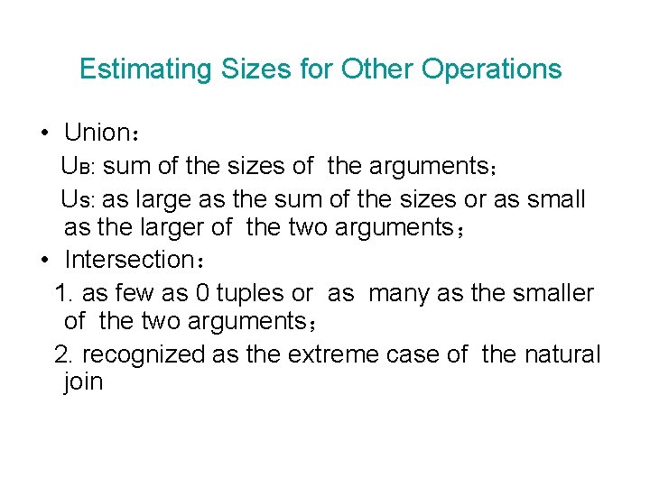
Estimating Sizes for Other Operations • Union： UB: sum of the sizes of the arguments； Us: as large as the sum of the sizes or as small as the larger of the two arguments； • Intersection： 1. as few as 0 tuples or as many as the smaller of the two arguments； 2. recognized as the extreme case of the natural join

• Difference： R-S: [T(R)+(T(R)-T(S)]/2=T(R)-T(S)/2 • Duplicate Eliminationδ (R) ： 1. (1+T(R))/2 2. V(R, a 1)*V(R, a 2)*…*V(R, an) • Grouping and Aggregation 1. Product of V(R, A)’s，A is grouping attribute； 2. [1+T(R)]/2

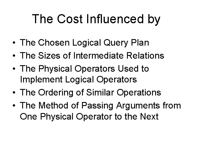
The Cost Influenced by • The Chosen Logical Query Plan • The Sizes of Intermediate Relations • The Physical Operators Used to Implement Logical Operators • The Ordering of Similar Operations • The Method of Passing Arguments from One Physical Operator to the Next

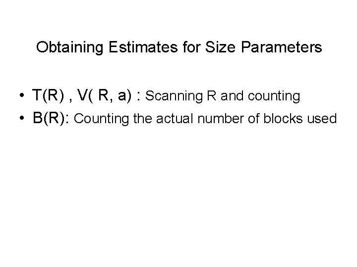
Obtaining Estimates for Size Parameters • T(R) , V( R, a) : Scanning R and counting • B(R): Counting the actual number of blocks used

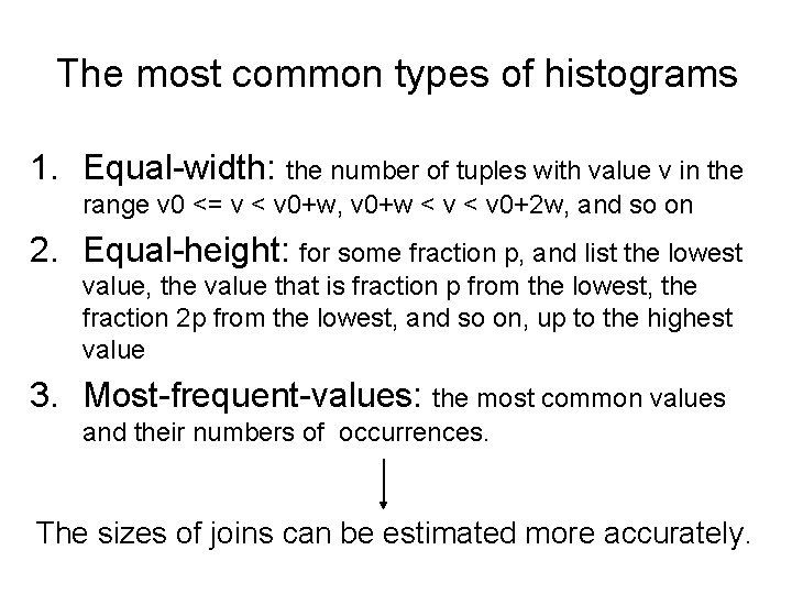
The most common types of histograms 1. Equal-width: the number of tuples with value v in the range v 0 <= v < v 0+w, v 0+w < v 0+2 w, and so on 2. Equal-height: for some fraction p, and list the lowest value, the value that is fraction p from the lowest, the fraction 2 p from the lowest, and so on, up to the highest value 3. Most-frequent-values: the most common values and their numbers of occurrences. The sizes of joins can be estimated more accurately.

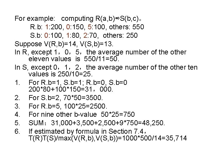
For example: computing R(a, b)∞S(b, c)。 R. b: 1: 200, 0: 150, 5: 100, others: 550 S. b: 0: 100, 1: 80, 2: 70, others: 250 Suppose V(R, b)=14, V(S, b)=13. In R, except 1，0，5，the average number of the other eleven values is 550/11=50. In S, except 0，1，2，the average number of the other ten values is 250/10=25. 1. For R. b=1, S. b=1; R. b=0, S. b=0 200*80+100*150=31，000. 2. For S. b=2, 70*50=3500. 3. For R. b=5, 100*25=2500. 4. For nine other b-value 50*25=750 5. SUM： 31, 000+3, 500+2, 500+9*750=48, 250. 6. If estimated by formula in Section 7. 4， T(R)T(S)/max(V(R, b), V(S, b))=1000*500/14=35, 714

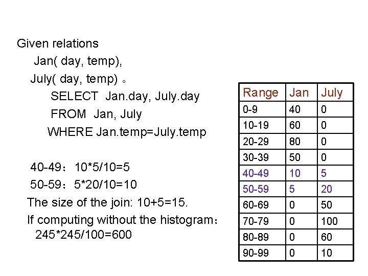
Given relations Jan( day, temp), July( day, temp) 。 SELECT Jan. day, July. day FROM Jan, July WHERE Jan. temp=July. temp 40 -49： 10*5/10=5 50 -59： 5*20/10=10 The size of the join: 10+5=15. If computing without the histogram： 245*245/100=600 Range Jan July 0 -9 40 0 10 -19 60 0 20 -29 80 0 30 -39 50 0 40 -49 10 5 50 -59 5 20 60 -69 0 50 70 -79 0 100 80 -89 0 60 90 -99 0 10

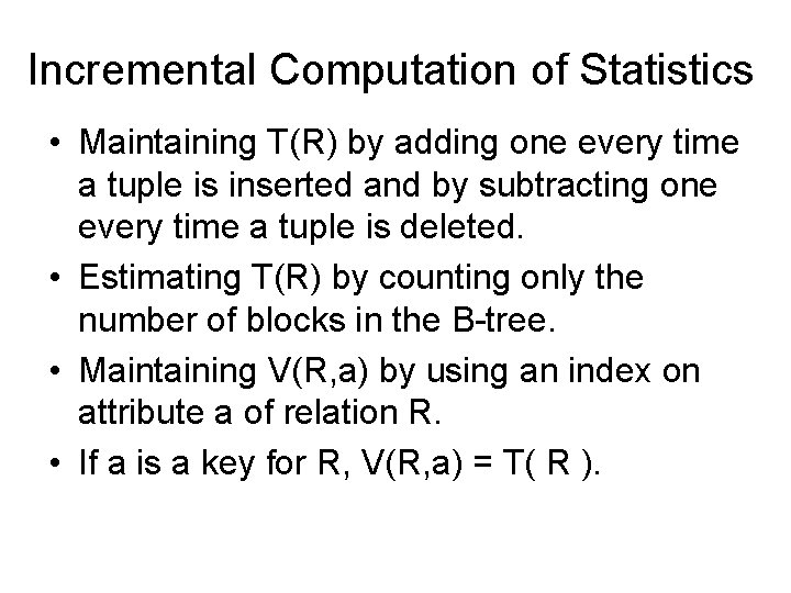
Incremental Computation of Statistics • Maintaining T(R) by adding one every time a tuple is inserted and by subtracting one every time a tuple is deleted. • Estimating T(R) by counting only the number of blocks in the B-tree. • Maintaining V(R, a) by using an index on attribute a of relation R. • If a is a key for R, V(R, a) = T( R ).

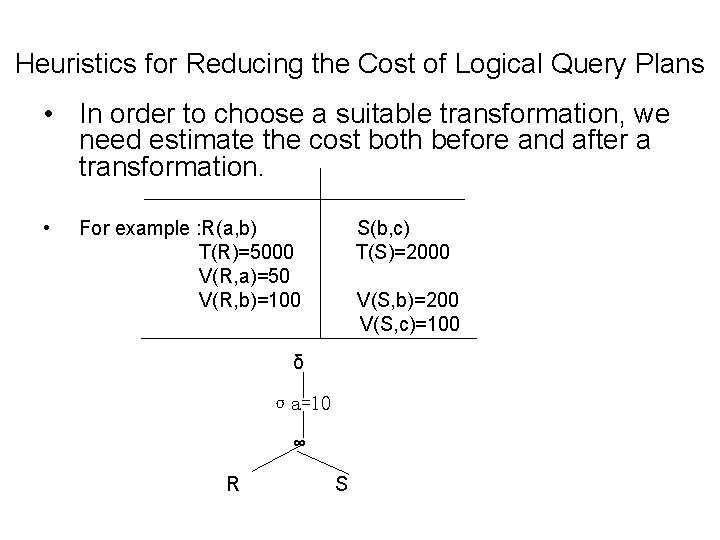
Heuristics for Reducing the Cost of Logical Query Plans • In order to choose a suitable transformation, we need estimate the cost both before and after a transformation. • For example : R(a, b) T(R)=5000 V(R, a)=50 V(R, b)=100 S(b, c) T(S)=2000 V(S, b)=200 V(S, c)=100 δ σa=10 ∞ R S

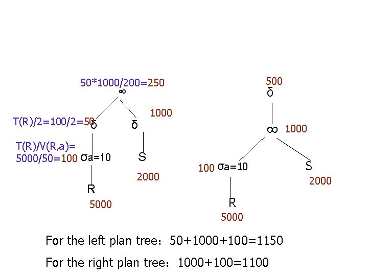
500 50*1000/200=250 δ ∞ T(R)/2=100/2=50δ T(R)/V(R, a)= 5000/50=100 σa=10 R 5000 δ 1000 S 2000 ∞ 1000 100 σa=10 S 2000 R 5000 For the left plan tree： 50+100=1150 For the right plan tree： 1000+100=1100

Approaches to Enumerating Physical Plans • Exhaustive • Top-down • Bottom-up

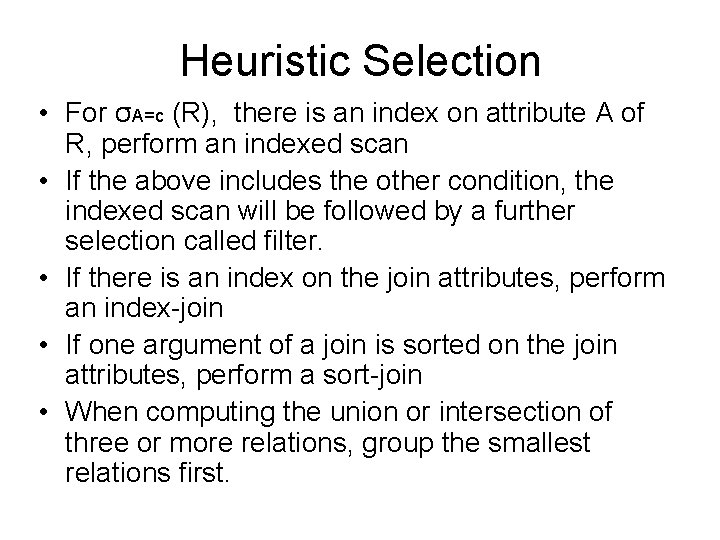
Heuristic Selection • For σA=c (R), there is an index on attribute A of R, perform an indexed scan • If the above includes the other condition, the indexed scan will be followed by a further selection called filter. • If there is an index on the join attributes, perform an index-join • If one argument of a join is sorted on the join attributes, perform a sort-join • When computing the union or intersection of three or more relations, group the smallest relations first.

Branch-and-Bound Plan Enumeration • Use heuristics to find a good physical plan with cost C and then explore the space of physical query plans. • Eliminate any plan having the subquery with cost greater than C. • Replace the current plan with the new plan having cost less than C.

Hill Climbing • Use heuristics to find a good physical plan. • Make small changes to the plan to find “nearby” plans that have lower cost by (1) replacing one method for an operator by another. (2) reordering joins by using the associative and/or commutative laws.

Dynamic Programming • Variation of the general bottom-up strategy • Keep for each subexpression only the plan of least cost. • Only the best plan for each subexpression is considered during constructing the plans for a larger subexpression.

Selinger-Style Optimization • Keep for each subexpression not only the plan of least cost, but certain other plans that have higher cost but produce a result that is sorted in an order that may be useful higher up in the expression tree. • Produce optimal overall plans from plans that are not optimal for certain subexpressions.

Choosing an Order for Joins Selecting an order for the (natural) join of three or more relations. The same ideas can be applied to other binary operations like union or intersection.

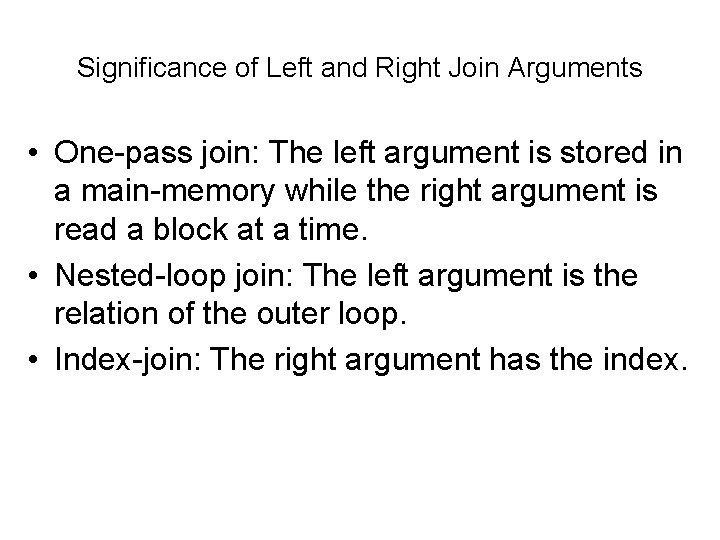
Significance of Left and Right Join Arguments • One-pass join: The left argument is stored in a main-memory while the right argument is read a block at a time. • Nested-loop join: The left argument is the relation of the outer loop. • Index-join: The right argument has the index.

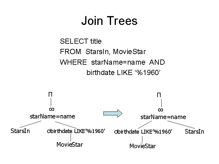
Join Trees SELECT title FROM Stars. In, Movie. Star WHERE star. Name=name AND birthdate LIKE ‘%1960’ Π Π ∞ star. Name=name Stars. In σbirthdate LIKE’%1960’ Movie. Star ∞ star. Name=name σbirthdate LIKE’%1960’ Movie. Stars. In

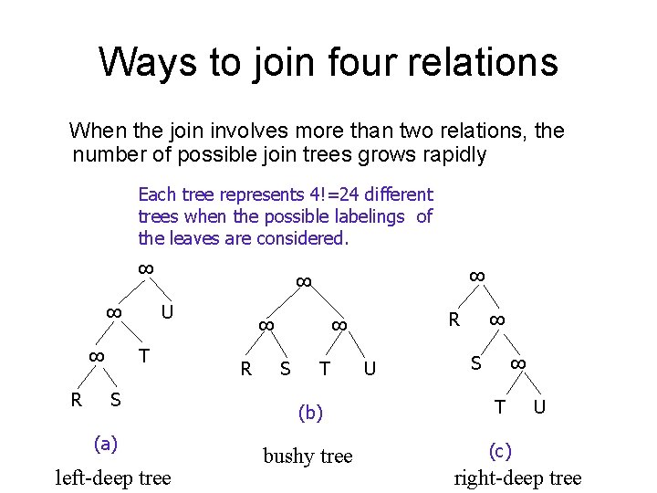
Ways to join four relations When the join involves more than two relations, the number of possible join trees grows rapidly Each tree represents 4!=24 different trees when the possible labelings of the leaves are considered. ∞ ∞ ∞ R ∞ ∞ U T S (a) left-deep tree ∞ R R ∞ S T U ∞ S ∞ (b) T bushy tree (c) U right-deep tree

Left-Deep Join Trees Only considering left-deep join trees has the following advantages • Limit the search space • Interact well with common join algorithms

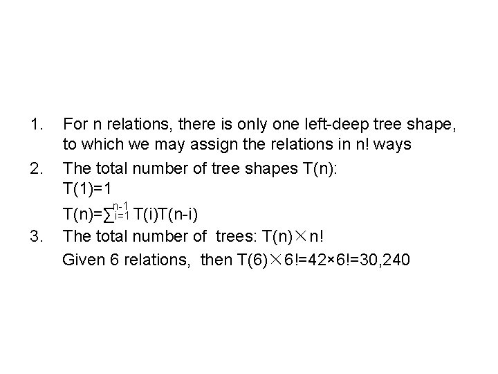
1. 2. For n relations, there is only one left-deep tree shape, to which we may assign the relations in n! ways The total number of tree shapes T(n): T(1)=1 n-1 T(n)=∑i=1 T(i)T(n-i) 3. The total number of trees: T(n)×n! Given 6 relations, then T(6)× 6!=42× 6!=30, 240

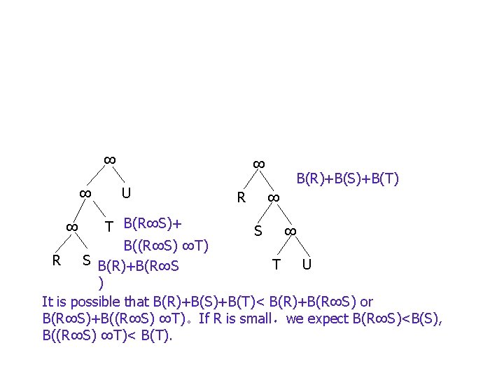
∞ ∞ ∞ U R B(R)+B(S)+B(T) ∞ T B(R∞S)+ S ∞ B((R∞S) ∞T) R S B(R)+B(R∞S T U ) It is possible that B(R)+B(S)+B(T)< B(R)+B(R∞S) or B(R∞S)+B((R∞S) ∞T)。If R is small，we expect B(R∞S)<B(S), B((R∞S) ∞T)< B(T). ∞

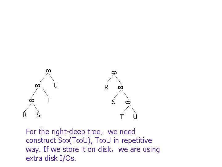
∞ ∞ ∞ R U T S ∞ R ∞ S ∞ T U For the right-deep tree，we need construct S∞(T∞U), T∞U in repetitive way. If we store it on disk，we are using extra disk I/Os.

Dynamic Programming to Select a Join Order and Grouping • • • Three choices to pick an order for the join of many relations. Consider them all Consider a subset Use a heuristic to pick one

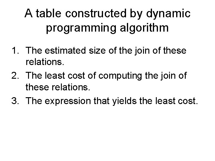
A table constructed by dynamic programming algorithm 1. The estimated size of the join of these relations. 2. The least cost of computing the join of these relations. 3. The expression that yields the least cost.

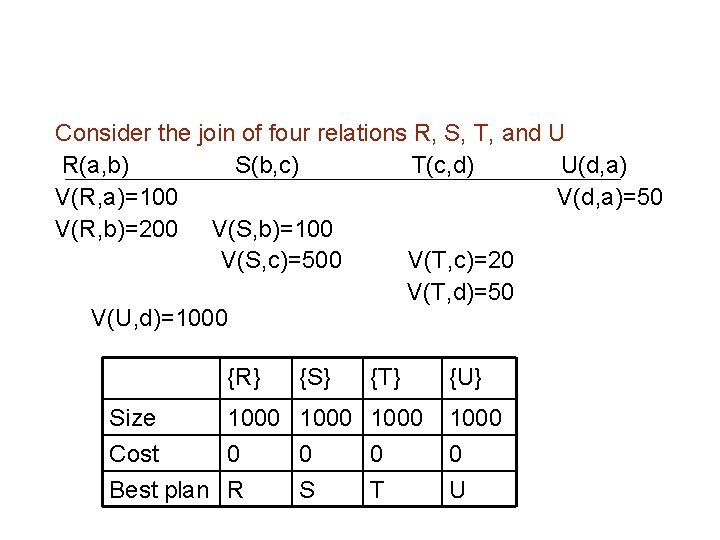
Consider the join of four relations R, S, T, and U R(a, b) S(b, c) T(c, d) U(d, a) V(R, a)=100 V(d, a)=50 V(R, b)=200 V(S, b)=100 V(S, c)=500 V(T, c)=20 V(T, d)=50 V(U, d)=1000 {R} {S} {T} Size 1000 Cost 0 0 0 Best plan R S T {U} 1000 0 U

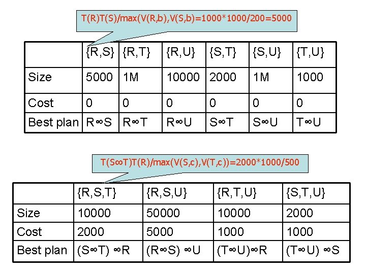
T(R)T(S)/max(V(R, b), V(S, b)=1000*1000/200=5000 {R, S} {R, T} {R, U} Size 5000 1 M Cost 0 0 Best plan R∞S R∞T {S, T} {S, U} {T, U} 10000 2000 1 M 1000 0 0 R∞U S∞T S∞U T(S∞T)T(R)/max(V(S, c), V(T, c))=2000*1000/500 {R, S, T} {R, S, U} {R, T, U} {S, T, U} Size 10000 50000 10000 2000 Cost 2000 5000 1000 (R∞S) ∞U (T∞U)∞R (T∞U) ∞S Best plan (S∞T) ∞R

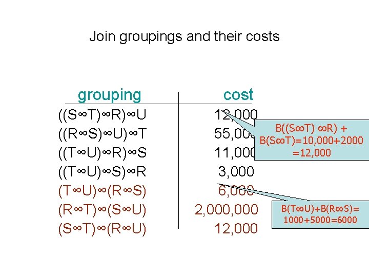
Join groupings and their costs grouping ((S∞T)∞R)∞U ((R∞S)∞U)∞T ((T∞U)∞R)∞S ((T∞U)∞S)∞R (T∞U)∞(R∞S) (R∞T)∞(S∞U) (S∞T)∞(R∞U) cost 12, 000 ∞T) ∞R) + 55, 000 B(SB((S ∞T)=10, 000+2000 =12, 000 11, 000 3, 000 6, 000 B(T∞U)+B(R∞S)= 2, 000 1000+5000=6000 12, 000

Dynamic Programming With More Detailed Cost Functions • Use Disk I/O as the cost measure • Compute the cost of R 1 ∞ R 2 by summing the cost of R 1, the cost of R 2, and the least cost of joining these two relations. • Dynamic programming based on the Selinger-style optimization.

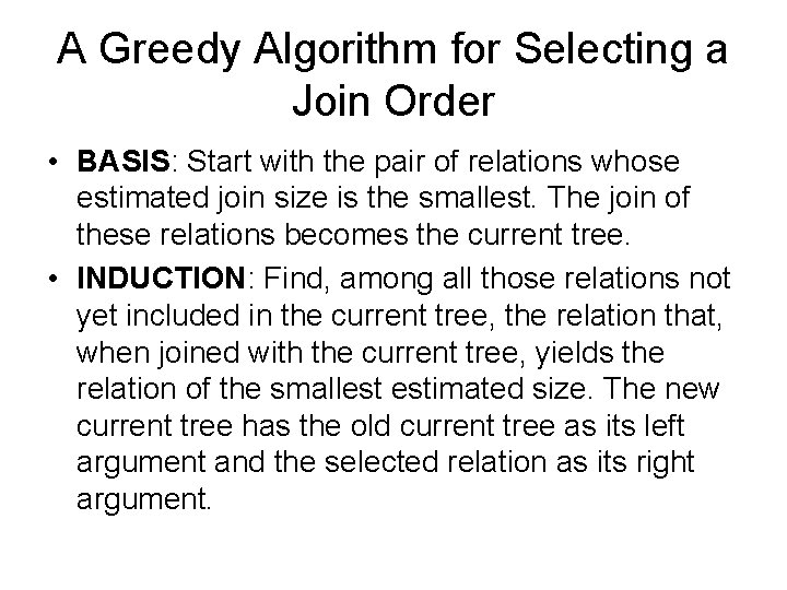
A Greedy Algorithm for Selecting a Join Order • BASIS: Start with the pair of relations whose estimated join size is the smallest. The join of these relations becomes the current tree. • INDUCTION: Find, among all those relations not yet included in the current tree, the relation that, when joined with the current tree, yields the relation of the smallest estimated size. The new current tree has the old current tree as its left argument and the selected relation as its right argument.

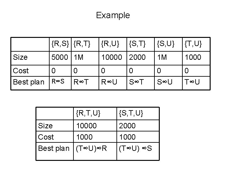
Example Size {R, S} {R, T} {R, U} 5000 1 M Cost 0 Best plan R∞S 0 R∞T {S, U} {T, U} 10000 2000 1 M 1000 0 R∞U 0 S∞U 0 T∞U {R, T, U} Size 10000 Cost 1000 Best plan (T∞U)∞R {S, T} 0 S∞T {S, T, U} 2000 1000 (T∞U) ∞S

Completing the Physical-Query. Plan Selection 1. Selection of algorithms to implement the operations of the query plan. 2. Decision regarding when intermediate results will be materialized and when they will be pipelined 3. Notation for physical-query-plan operators.

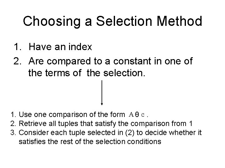
Choosing a Selection Method 1. Have an index 2. Are compared to a constant in one of the terms of the selection. 1. Use one comparison of the form Ａθｃ. 2. Retrieve all tuples that satisfy the comparison from 1 3. Consider each tuple selected in (2) to decide whether it satisfies the rest of the selection conditions

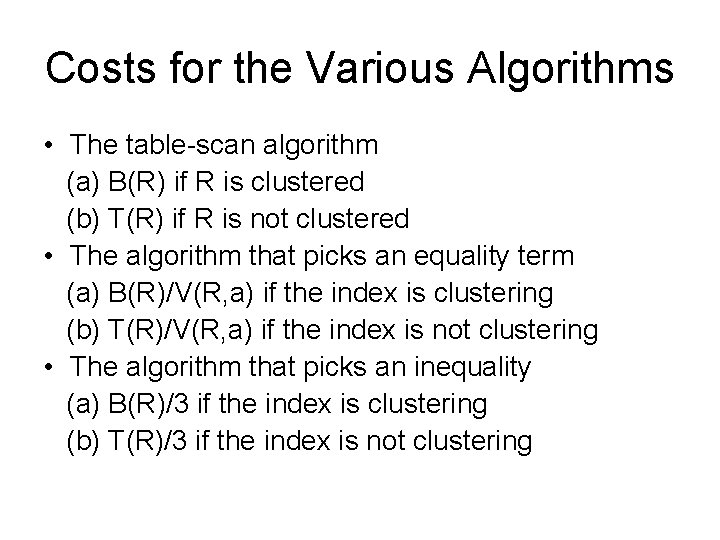
Costs for the Various Algorithms • The table-scan algorithm (a) B(R) if R is clustered (b) T(R) if R is not clustered • The algorithm that picks an equality term (a) B(R)/V(R, a) if the index is clustering (b) T(R)/V(R, a) if the index is not clustering • The algorithm that picks an inequality (a) B(R)/3 if the index is clustering (b) T(R)/3 if the index is not clustering

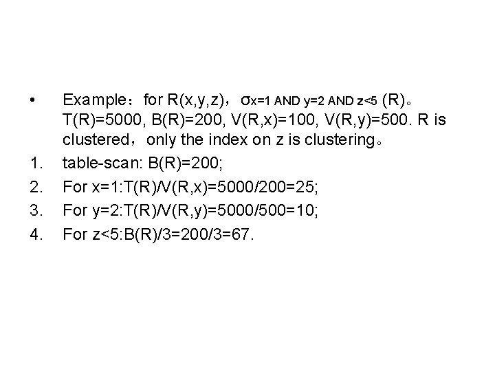
• 1. 2. 3. 4. Example：for R(x, y, z)，σx=1 AND y=2 AND z<5 (R)。 T(R)=5000, B(R)=200, V(R, x)=100, V(R, y)=500. R is clustered，only the index on z is clustering。 table-scan: B(R)=200; For x=1: T(R)/V(R, x)=5000/200=25; For y=2: T(R)/V(R, y)=5000/500=10; For z<5: B(R)/3=200/3=67.

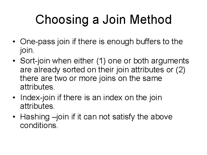
Choosing a Join Method • One-pass join if there is enough buffers to the join. • Sort-join when either (1) one or both arguments are already sorted on their join attributes or (2) there are two or more joins on the same attributes. • Index-join if there is an index on the join attributes. • Hashing –join if it can not satisfy the above conditions.

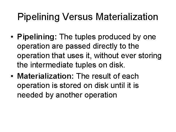
Pipelining Versus Materialization • Pipelining: The tuples produced by one operation are passed directly to the operation that uses it, without ever storing the intermediate tuples on disk. • Materialization: The result of each operation is stored on disk until it is needed by another operation

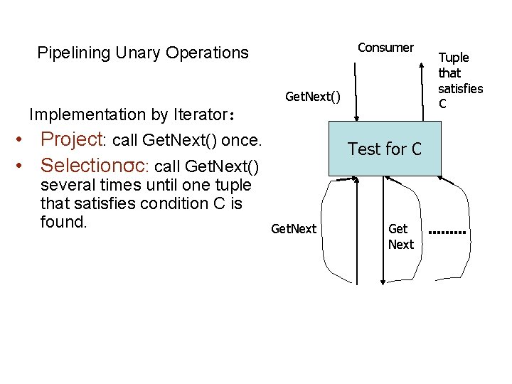
Consumer Pipelining Unary Operations Implementation by Iterator： Get. Next() • Project: call Get. Next() once. • Selectionσc: call Get. Next() several times until one tuple that satisfies condition C is found. Test for C Get. Next Get Next Tuple that satisfies C

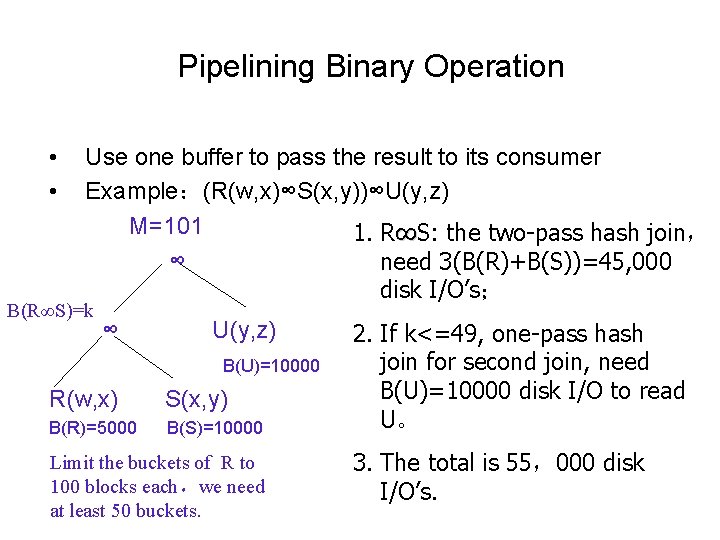
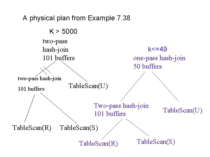
Pipelining Binary Operation • • Use one buffer to pass the result to its consumer Example：(R(w, x)∞S(x, y))∞U(y, z) M=101 1. R∞S: the two-pass hash join， ∞ need 3(B(R)+B(S))=45, 000 disk I/O’s； B(R∞S)=k ∞ U(y, z) B(U)=10000 R(w, x) S(x, y) B(R)=5000 B(S)=10000 Limit the buckets of R to 100 blocks each，we need at least 50 buckets. 2. If k<=49, one-pass hash join for second join, need B(U)=10000 disk I/O to read U。 3. The total is 55，000 disk I/O’s.

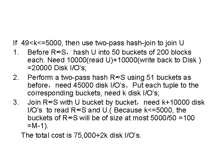
If 49<k<=5000, then use two-pass hash-join to join U 1. Before R∞S，hash U into 50 buckets of 200 blocks each. Need 10000(read U)+10000(write back to Disk ) =20000 Disk I/O’s; 2. Perform a two-pass hash R∞S using 51 buckets as before，need 45000 disk I/O’s。Put each tuple to the corresponding buckets, need k disk I/O’s; 3. Join R∞S with U bucket by bucket，need k+10000 disk I/O’s to read R∞S and U. ( Because k<=5000, the buckets of R∞S will be of size at most 5000/50 =100 =M-1). The total cost is 75, 000+2 k disk I/O’s.

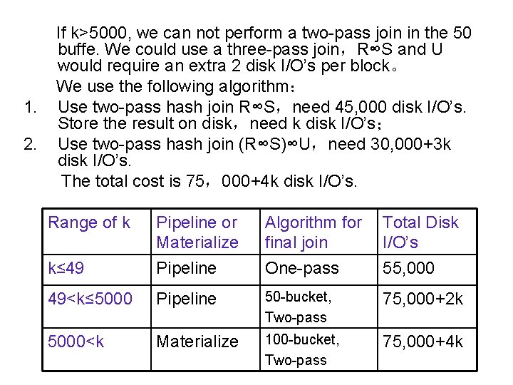
1. 2. If k>5000, we can not perform a two-pass join in the 50 buffe. We could use a three-pass join，R∞S and U would require an extra 2 disk I/O’s per block。 We use the following algorithm： Use two-pass hash join R∞S，need 45, 000 disk I/O’s. Store the result on disk，need k disk I/O’s； Use two-pass hash join (R∞S)∞U，need 30, 000+3 k disk I/O’s. The total cost is 75，000+4 k disk I/O’s. Range of k Pipeline or Materialize Algorithm for final join Total Disk I/O’s k≤ 49 Pipeline One-pass 55, 000 49<k≤ 5000 Pipeline 50 -bucket, Two-pass 75, 000+2 k 5000<k Materialize 100 -bucket, Two-pass 75, 000+4 k

Notation for Physical Query Plans • Each operator of the logical plan becomes one or more operators of the physical plan • Leaves (stored relations) of the logical plan become one of the scan operators applied to that relation. • Materialization would be indicated by a Store operator applied to the intermediate result.

Operators for leaves 1. 2. 3. 4. Each relation R that is a leaf operand of the logicalquery-plan tree will be replaced by a scan operator： Table. Scan(R) : All blocks holding tuples of R are read in arbitrary order. Sort. Scan(R, L): Tuples of R are read in order, sorted according to the attribute(s) on List L Index. Scan(R, C): C is a condition of the form Aθc， Tuples of R are accessed through an index on attribute A. Index. Scan(R, A)：A is an attribute of R. The entire relation R is retrieved via an index on R. A.

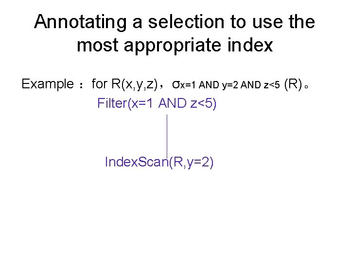
Physical Operators for Selection 1. Replace σc(R) with Filter (C) If R is intermediate relation，no other operator besides Filter is needed. If R is a stored or materialized relation，Table. Scan, Sort. Scan(L) are used to access R. 2. If condition C can be expressed as Aθc AND D，there is an index on R. A，then a) Use the operator Index. Scan(R, Aθc ) to access R； b) Use Filter(D) in place of the selectionσc(R).

• Physical Sort Operators： – Introduce Sort. Scan(R, L) which reads a stored relation R, and produces it sorted according to the list of attributes L。 • Other Relational-Algebra Operations: Replaced by a suitable physical operator： – The operation being performed； – Necessary parameters； – A general strategy for the algorithm: sort-based, hash-based, or in some joins, index-based； – A decision about the number of passes to be used ； – An anticipated number of buffers the operation will require

A physical plan from Example 7. 38 K > 5000 two-pass hash-join 101 buffers k<=49 one-pass hash-join 50 buffers two-pass hash-join 101 buffers Table. Scan(U) Two-pass hash-join 101 buffers Table. Scan(R) Table. Scan(U) Table. Scan(S) Table. Scan(R) Table. Scan(S)

Annotating a selection to use the most appropriate index Example ：for R(x, y, z)，σx=1 AND y=2 AND z<5 (R)。 Filter(x=1 AND z<5) Index. Scan(R, y=2)

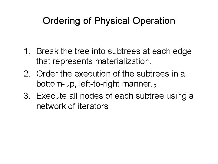
Ordering of Physical Operation 1. Break the tree into subtrees at each edge that represents materialization. 2. Order the execution of the subtrees in a bottom-up, left-to-right manner. ； 3. Execute all nodes of each subtree using a network of iterators

Exercises • • Ex 7. 1. 3, Ex 7. 2. 2 (b), (c) , (d) Ex 7. 3. 1 (c) , Ex 7. 3. 2 Ex 7. 4. 1 (c) , (d), (e), Ex 7. 5. 1 Ex 7. 6. 1, Ex 7. 7. 1 (b), (c)