Chapter 7 The Laplace Transform Consider the following
 System analysis")


 Laplace transform pairs Forward transform Inverse transform Complex domain Because of")
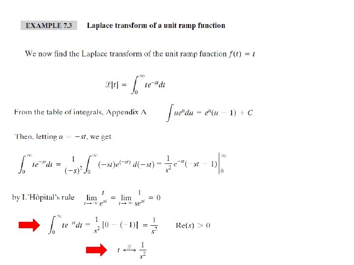
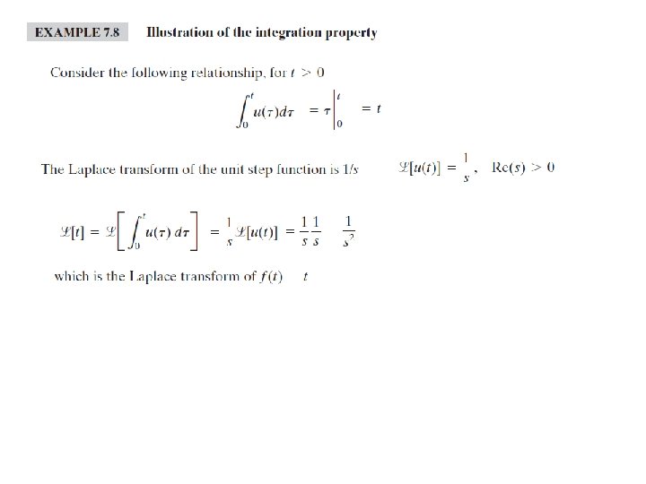
 Assuming the lower limit is 0 The value")


 for a cosine function Since")


 Since (Shift in time property)")


 Since")


 , D(s) are either")
 ( which is related to input) must be less than")
 must have real parts which are negative The poles must")
 ( It is very similar to the Fourier Transform Property")
 for this circuit is given by If v(t) = 12")
 = 12 u(t) Now using the Laplace Table 7. 2 to find i(t)")


")

")
 Let Y(s) be Laplace Transform of")


 into simple known forms Simple Factors")
 both side by (s+2) and set s =")

")

 Can be combined as")


- Slides: 67
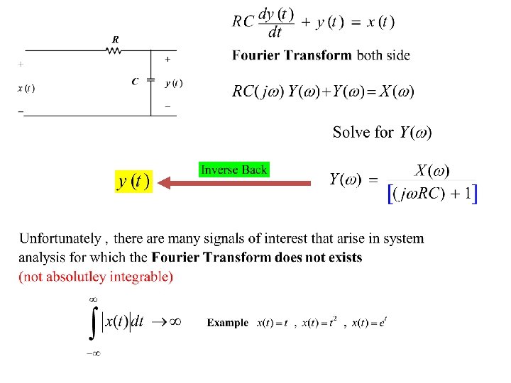
Chapter 7 The Laplace Transform Consider the following RC circuit ( System) System analysis in the time domain involves ( finding y(t)): Solving the differential equation OR Using the convolution integral Both Techniques can results in tedious ( ) ﻣﻤﻞ mathematical operation
Fourier Transform provided an alternative approach Differential Equation Inverse Back
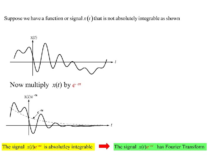
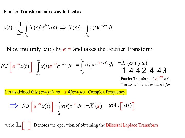
7. 1 DEFINITIONS OF LAPLACE TRANSFORMS The Laplace transform variable is complex This show that the bilateral Laplace transform of a signal can be interpreted as the Fourier transform of that signal multiplied by an exponential function
The inverse Laplace transform where This transform is usually called, simply, the Laplace transform , the subscript b dropped Laplace transform pairs
Unilateral (single sided) Laplace transform pairs Forward transform Inverse transform Complex domain Because of the difficulty in evaluating the complex inversion integral Simpler procedure to find the inverse of Laplace Transform (i. e f(t) ) will be presented later Using Properties and table of known transform ( similar to Fourier)
Laplace Transform for an impulse d(t) Assuming the lower limit is 0 The value of s make no difference Region of Convergence We also can drive it from the shifting in time property that will be discussed later
For this to converge then
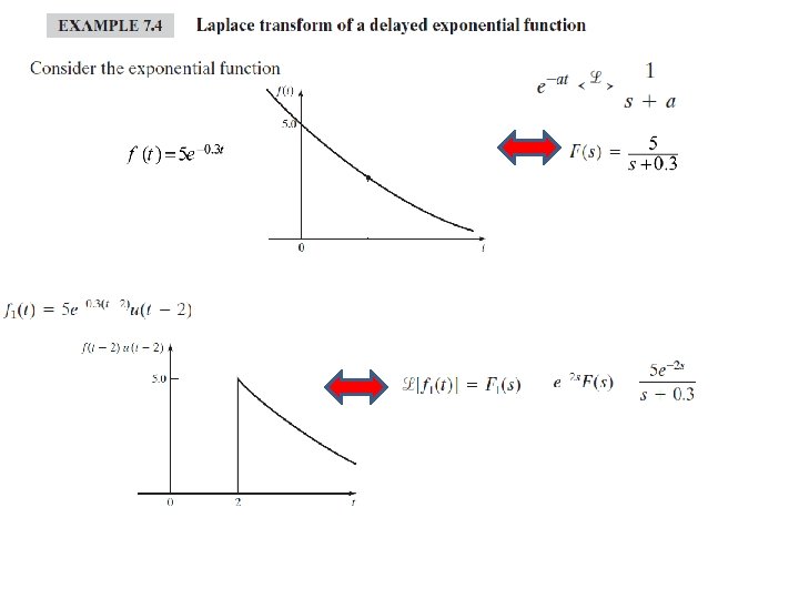
We derive the Laplace transform of the exponential function
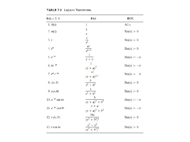
A short table of Laplace transforms is constructed from Examples 7. 1 and 7. 2 and is given as Table 7. 2
We know derive the Laplace Transform (LT) for a cosine function Since
Proof Let s*= s+a
Example Since Then Similarly
Real Shifting Let
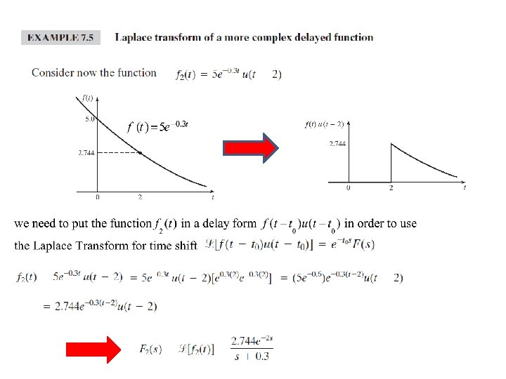
It is sometimes necessary to construct complex waveforms from simpler waveforms
(See example 7. 3) Since (Shift in time property)
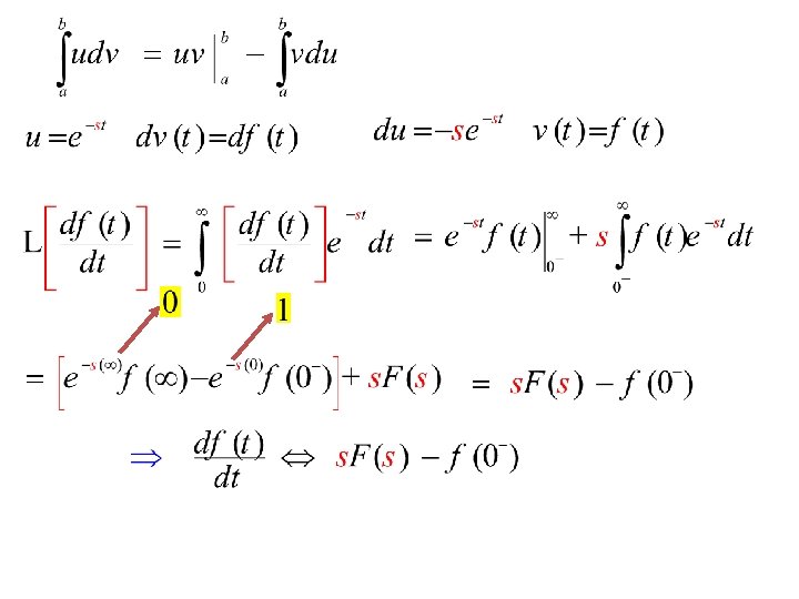
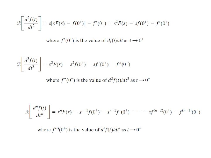
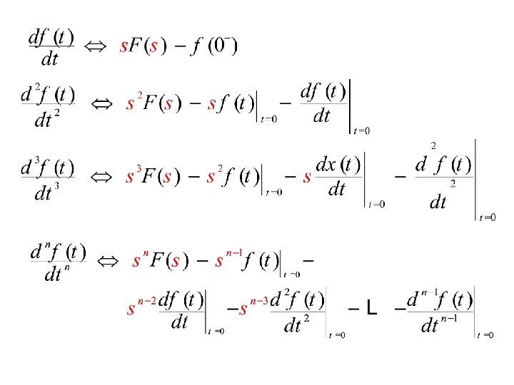
Transform of Derivatives
Proof Integrating by parts,
Proof
find the Laplace transforms of the following integrals:
Proof (See the book) Since
7. 6 Response of LTI Systems Transfer Functions Consider the following circuit We want a relation (an equation) between the input x(t) and output y(t) KVL
Writing the differential equation as
Real coefficients, non negative which results from system components R, L, C
In general, are real, non negative which results from system components R, L, C Now if we take the Laplace Transform of both side (Assuming Zero initial Conditions) We now define the transfer function H(s) ,
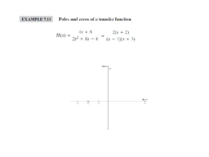
are real, non negative The roots of the polynomials N(s) , D(s) are either real or occur in complex conjugate The roots of N(s) are referred to as the zero of H(s) ( H(s) = 0 ) The roots of D(s) are referred to as the pole of H(s) ( H(s) = ± ∞ )
The Degree of N(s) ( which is related to input) must be less than or Equal of D(s) ( which is related to output) for the system to be Bounded-input, bounded-output (BIBO) Example : Using polynomial division , we obtain Now assume the input x(t) = u(t) (bounded input) We see that for finite bounded Input (i. e x(t) =u(t) ) We get an infinite (unbounded) output
The poles of H(s) must have real parts which are negative The poles must lie in the left half of the s-plan
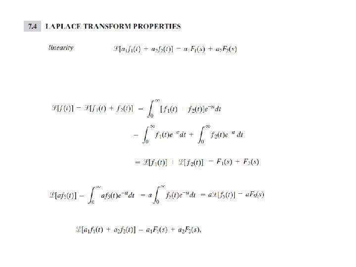
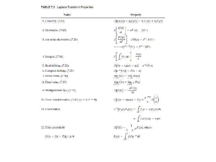
Proof (See the book) ( It is very similar to the Fourier Transform Property )
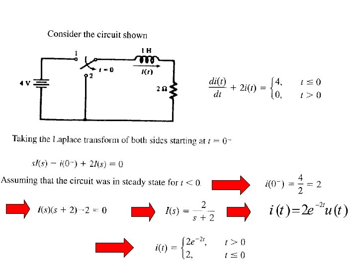
The loop equation (KVL) for this circuit is given by If v(t) = 12 u(t) , find i(t) ?
v(t) = 12 u(t) Now using the Laplace Table 7. 2 to find i(t) The inverse transform, from Table 7. 2
Source Transformation
Source Transformation
Example Using Laplace Transform Method find i(t)
KVL
( Imaginary Roots)
Inversion of Rational Function ( Inverse Laplace Transform) Let Y(s) be Laplace Transform of some function y(t). We want to find y(t) without using the inversion formula. We want to find y(t) using the Laplace Transform known table and properties Objective : Put Y(s) in a form or a sum of forms that we know it is in the Laplace Transform Table Y(s) in general is a ratio of two polynomials Rational Function
When the degree of the numerator of rational function is less the Degree of the dominator Proper Rational Function Highest Degree is 2 Highest Degree is 3
Examples of proper rational Functions Examples of not proper rational Functions However we can obtain a proper rational Function through long division
We will discuss different techniques of factoring Y(s) into simple known forms Simple Factors If we check the Table , we see there is no form similar to Y(s) However if we expand Y(s) in partial fractions: Are available on the Table Next we develop Techniques of finding A and B
Heavisdie’s Expansion Theorem Multiply ( ) both side by (s+2) and set s = -2 Similarly Multiply both side by (s +8) and set s = -8
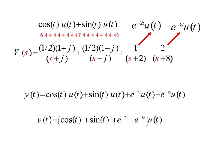
Imaginary Roots Using Heavisdie’s Expansions, by multiplying the left hand side and Right hand side by the factors and substitute We obtain respectively
From Table Can be inverted in two methods: (a)
combine
(b) Can be combined as
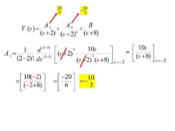
Repeated Linear Factor If Then its partial fraction Were
Repeated Linear Factor Let Also A 2 can be found using Heavisdie’s by multiplying both sides by B can be found using Heavisdie’s by multiplying both sides by Then
To find B , we use Heaviside
Repeated Linear Factor Let Then Can be found using Heaviside’s expansion
A 1 Can be found using Heaviside differentiation techniques