Chapter 7 Supervised Machine Learning Textbook Artificial Intelligence

Chapter 7 Supervised Machine Learning Textbook: Artificial Intelligence Foundations of Computational Agents, 2 nd Edition, David L. Poole and Alan K Mackworth, Cambridge University Press, 2018. Asst. Prof. Dr. Anilkumar K. G 1
Overview • The ability to learn is essential to any intelligent agent. • Learning is the ability of an agent to improve its behavior based on experience and this could mean: – The range of behaviors is expanded; the agent can do more. – The accuracy on tasks is improved; the agent can do things better. – The speed is improved; the agent can do things faster. • This lecture section considers the problem of making a prediction as supervised learning: – given a set of training examples made up of input–output pairs, predict the output of a new example (only the inputs are given). Asst. Prof. Dr. Anilkumar K. G 2
Learning Issues • The following components are part of any learning problem: • Task: The behavior or task that is being improved • Data: The experiences (a set of numerical values) that are used to improve performance in the task, in the form of a sequence of examples • Measure of improvement: How the improvement from learning is measured – for example, new skills that were not present initially, increasing accuracy in prediction, or improved speed Asst. Prof. Dr. Anilkumar K. G 3
Learning Issues - Task • The most commonly studied learning task is supervised learning: – From some input features and target features, generates a set of training examples, predict the value of target features for a new example with only input features. – This is called classification when the target features are discrete • Discrete data can take on only integer values – and is called regression when the target features are continuous. • For instance the number of liver patients treated by a hospital each year is discrete but their weights are continuous Asst. Prof. Dr. Anilkumar K. G 4
Learning Issues - Task • Other learning tasks include learning classifications when the examples do not have targets defined (called unsupervised learning) • Learning what to do based on rewards and punishments (called reinforcement learning) • Learning to reason faster (called analytic learning) • Learning richer representations such as logic programs (called inductive logic programming) Asst. Prof. Dr. Anilkumar K. G 5
Learning Issues - Feedback • Learning tasks can be characterized by the feedback given to the learner • In supervised learning, what has to be learned is specified for each example: • Supervised classification occurs when a trainer provides the classification for each example. • Supervised learning of actions occurs when the agent is given immediate feedback about the value of each action. • Unsupervised learning occurs when no classifications are given and the learner must discover categories and regularities within the data by itself. Asst. Prof. Dr. Anilkumar K. G 6
Learning Issues - Representation • For an agent its experiences must affect the agent’s internal representation. – This internal representation could be the raw experiences themselves – The problem of inferring an internal representation based on examples is called induction which is deriving consequences of a KB. • Much of machine learning is studied in the context of particular representations (e. g. , decision trees, neural networks, or case bases). Asst. Prof. Dr. Anilkumar K. G 7
Learning Issues - Online and offline • In offline learning, all of the training examples are available to an agent before it needs to act. • In online learning, training examples arrive as the agent is acting – An agent that learns online requires some representation of its previously seen examples before it has seen all of its examples. – As new examples are observed, the agent must update its representation. • Active learning is a form of online learning in which the agent acts to acquire useful examples from which to learn Asst. Prof. Dr. Anilkumar K. G 8
Learning Issues - Measuring success • Learning is defined in terms of improving performance based on some measure. • To know whether an agent has learned, we must define a measure of success. – The measure of success is usually not how well the agent performs on the training data (seen data), but how well the agent performs for new data (unseen data). • In classification, measuring successes is not based on classification of all training examples correctly – In classification, success in learning is judged based on correctly classifying the unseen examples. Asst. Prof. Dr. Anilkumar K. G 9
Learning Issues - Measuring success • The learner must generalize to classify the unseen examples. • A standard way to evaluate a learning procedure is to divide the examples into training examples and test examples – A representation is built using the training examples, and the predictive accuracy is measured on the test examples. – To properly evaluate the method, the test cases should not be known while the training is occurring. Asst. Prof. Dr. Anilkumar K. G 10
Learning Issues - Bias • The tendency to prefer one hypothesis over another is called a bias – For example, consider agents N and P and it is saying that a hypothesis is better than N’s or P’s hypothesis – Both N and P accurately predict all of the data given – but is something external to the data. – Without a bias, an agent will not be able to make any predictions on unseen examples. Asst. Prof. Dr. Anilkumar K. G 11
Learning Issues - Learning as search • Given a representation and a bias, the problem of learning can be reduced as a search – Learning is a search through the space of possible representations, trying to find the representation or representations that best fits the data given the bias. – Nearly all of the search techniques used in machine learning can be seen as forms of local search through a space of representations. – The definition of the learning algorithm then becomes one of defining the search space, the evaluation function, and the search method. Asst. Prof. Dr. Anilkumar K. G 12
Supervised Learning • Supervised learning is based on a set of examples: a set of features partitioned into input features and target features. – The aim is to predict the values of the target features from the input features. – A feature is a function from examples into a value: If e is an example, and F is a feature, F(e) is the value of feature F for example e. • If e is an example of a training set, and F is a feature, then val(e, F) be the value of feature F in example e. – The domain of a feature is the set of values it can return. • Note that this is the range of the function, but is traditionally called the domain. Asst. Prof. Dr. Anilkumar K. G 13
Supervised Learning • In a supervised learning task, the learner is given: – a set of input features, X 1, . . . , Xn; – a set of target features, Y 1, . . . , Yk; – a set of training examples, where the values for the input features and the target features are given for each example; and – a set of test examples, where only the values for the input features (it is the unseen data and is not from the training example) are given. • The aim is to predict the values of the target features for the unseen examples. Asst. Prof. Dr. Anilkumar K. G 14
Supervised Learning • Example 7. 1: Figure 7. 1 shows training examples (seen data) and test example (unseen data) of a classification task. The aim is to predict whether a person reads an article posted to a threaded discussion website given properties of the article • The input features are Author, Thread, Length, and Where. Read. There is only one target feature, User. Action. • The domain of Author is {known, unknown}, the domain of Thread is {new, followup}, and so on. – There are eighteen seen data (e 1, …. , e 18). • In this dataset, Author(e 11)=unknown, Thread(e 11)= follow. Up, and User. Action(e 11) = skips. • There are two test examples, e 19 and e 20, where the user action is unknown. – The aim is to predict the user. Action for these two test examples. Asst. Prof. Dr. Anilkumar K. G 15
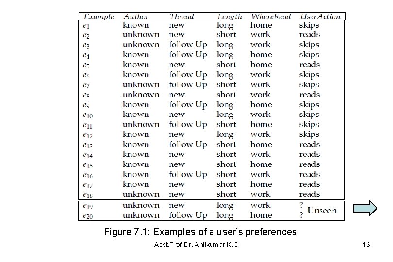
Figure 7. 1: Examples of a user’s preferences Asst. Prof. Dr. Anilkumar K. G 16
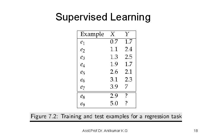
Supervised Learning • Example 7. 2: Figure 7. 2 shows some data for a regression task, where the aim is to predict the value of feature Y on examples for which the value of feature X is provided – This is a regression task because Y is a real-valued feature. – Predicting a value of Y for example e 8 is an interpolation problem, as its value for the input feature is between the values of the training examples. – Predicting a value of Y for the example e 9 is an extrapolation problem, because its X value is outside the range of the training examples. Asst. Prof. Dr. Anilkumar K. G 17
Supervised Learning Asst. Prof. Dr. Anilkumar K. G 18
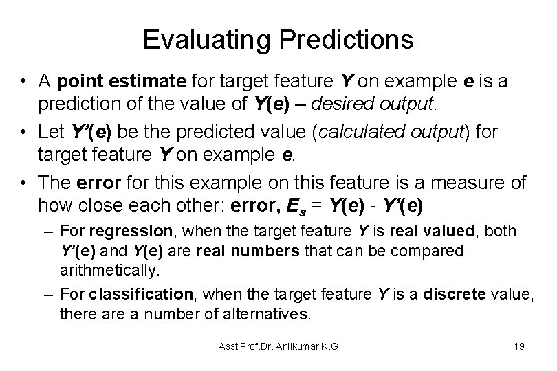
Evaluating Predictions • A point estimate for target feature Y on example e is a prediction of the value of Y(e) – desired output. • Let Y’(e) be the predicted value (calculated output) for target feature Y on example e. • The error for this example on this feature is a measure of how close each other: error, Es = Y(e) - Y’(e) – For regression, when the target feature Y is real valued, both Y’(e) and Y(e) are real numbers that can be compared arithmetically. – For classification, when the target feature Y is a discrete value, there a number of alternatives. Asst. Prof. Dr. Anilkumar K. G 19
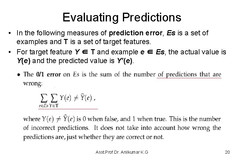
Evaluating Predictions • In the following measures of prediction error, Es is a set of examples and T is a set of target features. • For target feature Y ∈ T and example e ∈ Es, the actual value is Y(e) and the predicted value is Y’(e). Asst. Prof. Dr. Anilkumar K. G 20
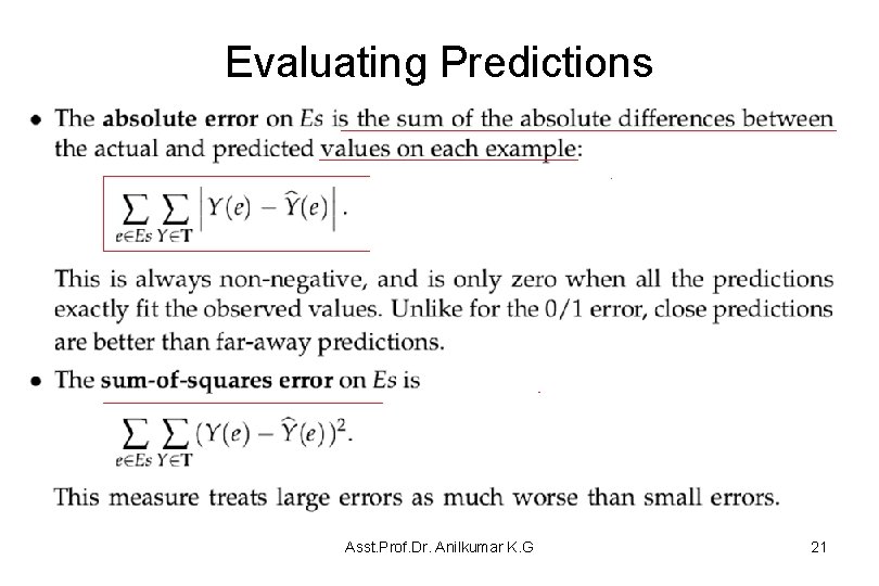
Evaluating Predictions Asst. Prof. Dr. Anilkumar K. G 21
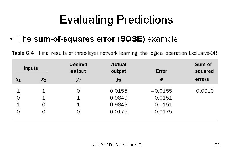
Evaluating Predictions • The sum-of-squares error (SOSE) example: Asst. Prof. Dr. Anilkumar K. G 22
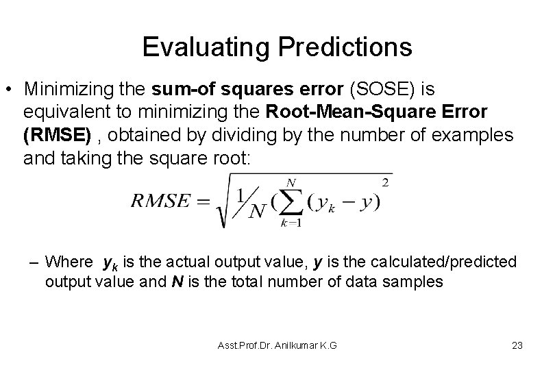
Evaluating Predictions • Minimizing the sum-of squares error (SOSE) is equivalent to minimizing the Root-Mean-Square Error (RMSE) , obtained by dividing by the number of examples and taking the square root: – Where yk is the actual output value, y is the calculated/predicted output value and N is the total number of data samples Asst. Prof. Dr. Anilkumar K. G 23
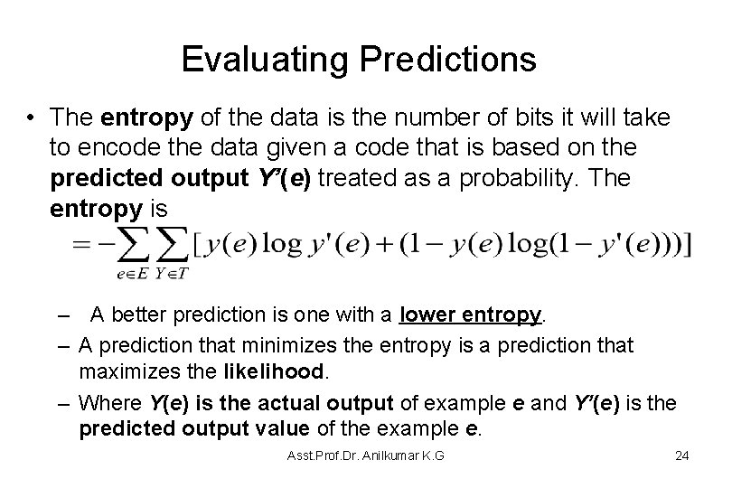
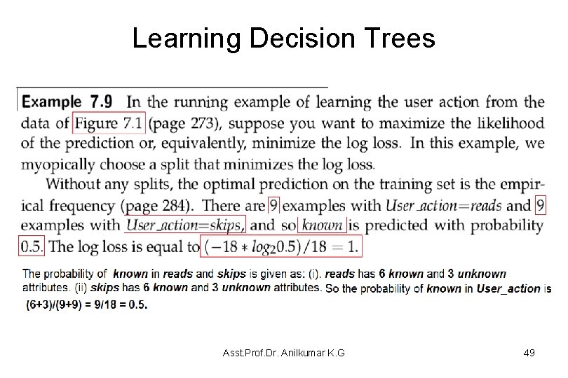
Evaluating Predictions • The entropy of the data is the number of bits it will take to encode the data given a code that is based on the predicted output Y’(e) treated as a probability. The entropy is – A better prediction is one with a lower entropy. – A prediction that minimizes the entropy is a prediction that maximizes the likelihood. – Where Y(e) is the actual output of example e and Y’(e) is the predicted output value of the example e. Asst. Prof. Dr. Anilkumar K. G 24
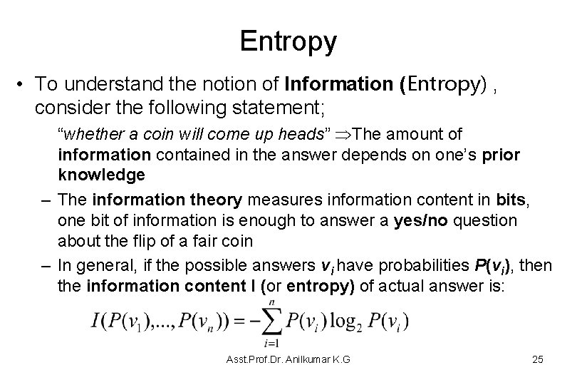
Entropy • To understand the notion of Information (Entropy) , consider the following statement; “whether a coin will come up heads” The amount of information contained in the answer depends on one’s prior knowledge – The information theory measures information content in bits, one bit of information is enough to answer a yes/no question about the flip of a fair coin – In general, if the possible answers vi have probabilities P(vi), then the information content I (or entropy) of actual answer is: Asst. Prof. Dr. Anilkumar K. G 25
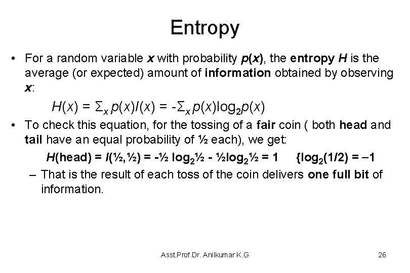
Entropy • For a random variable x with probability p(x), the entropy H is the average (or expected) amount of information obtained by observing x: H(x) = Σx p(x)I(x) = -Σx p(x)log 2 p(x) • To check this equation, for the tossing of a fair coin ( both head and tail have an equal probability of ½ each), we get: H(head) = I(½, ½) = -½ log 2½ - ½log 2½ = 1 {log 2(1/2) = 1 – That is the result of each toss of the coin delivers one full bit of information. Asst. Prof. Dr. Anilkumar K. G 26
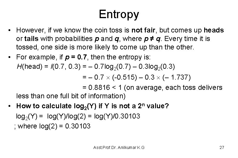
Entropy • However, if we know the coin toss is not fair, but comes up heads or tails with probabilities p and q, where p ≠ q. Every time it is tossed, one side is more likely to come up than the other. • For example, if p = 0. 7, then the entropy is: H(head) = I(0. 7, 0. 3) = – 0. 7 log 2(0. 7) – 0. 3 log 2(0. 3) = – 0. 7 (-0. 515) – 0. 3 (– 1. 737) = 0. 8816 < 1 (on average, each toss delivers less than one full bit of information) • How to calculate log 2(Y) if Y is not a 2 n value? log 2(Y) = log(Y)/log(2) = log(Y)/0. 30103 ; where log(2) = 0. 30103 Asst. Prof. Dr. Anilkumar K. G 27
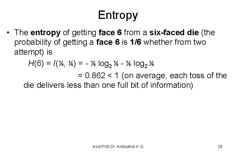
Entropy • The entropy of getting face 6 from a six-faced die (the probability of getting a face 6 is 1/6 whether from two attempt) is H(6) = I(⅙, ⅙) = - ⅙ log 2 ⅙ = 0. 862 < 1 (on average, each toss of the die delivers less than one full bit of information) Asst. Prof. Dr. Anilkumar K. G 28
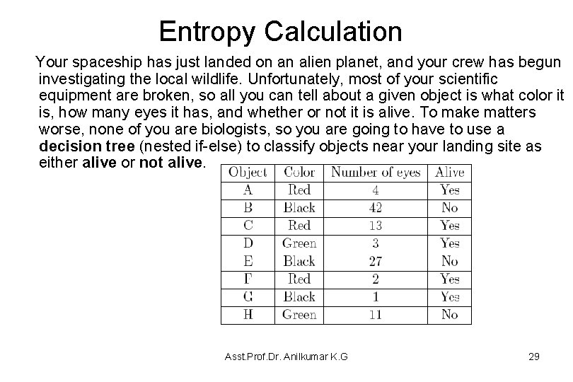
Entropy Calculation Your spaceship has just landed on an alien planet, and your crew has begun investigating the local wildlife. Unfortunately, most of your scientific equipment are broken, so all you can tell about a given object is what color it is, how many eyes it has, and whether or not it is alive. To make matters worse, none of you are biologists, so you are going to have to use a decision tree (nested if-else) to classify objects near your landing site as either alive or not alive. Asst. Prof. Dr. Anilkumar K. G 29
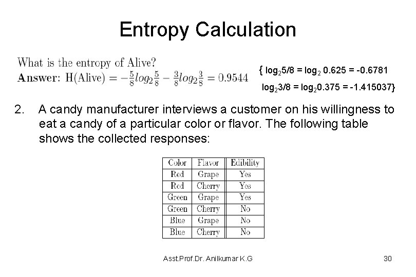
Entropy Calculation { log 25/8 = log 2 0. 625 = -0. 6781 log 23/8 = log 20. 375 = -1. 415037} 2. A candy manufacturer interviews a customer on his willingness to eat a candy of a particular color or flavor. The following table shows the collected responses: Asst. Prof. Dr. Anilkumar K. G 30
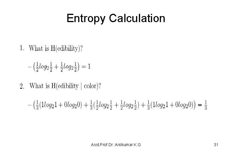
Entropy Calculation Asst. Prof. Dr. Anilkumar K. G 31
Types of Learning Errors • Not all errors are equal; the consequences of some errors may be much worse than others. – For example, it may be much worse to predict a patient does not have a disease that the patient actually has, so that the patient does not get appropriate treatment – Similarly it is predict that a patient has a disease the patient does not actually have, which will force the patient to undergo further unwanted tests. • The agent should choose the best prediction according to the costs associated with the errors. Asst. Prof. Dr. Anilkumar K. G 32
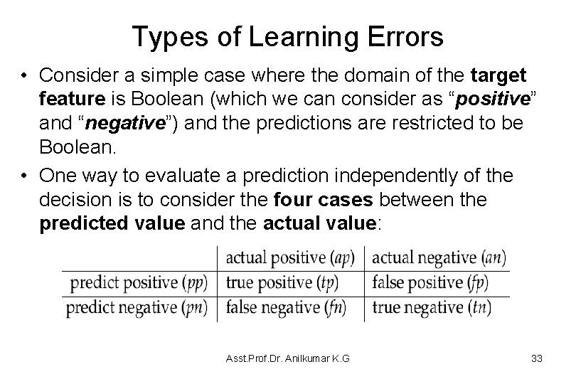
Types of Learning Errors • Consider a simple case where the domain of the target feature is Boolean (which we can consider as “positive” and “negative”) and the predictions are restricted to be Boolean. • One way to evaluate a prediction independently of the decision is to consider the four cases between the predicted value and the actual value: Asst. Prof. Dr. Anilkumar K. G 33
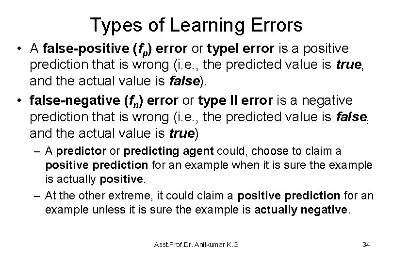
Types of Learning Errors • A false-positive (fp) error or type. I error is a positive prediction that is wrong (i. e. , the predicted value is true, and the actual value is false). • false-negative (fn) error or type II error is a negative prediction that is wrong (i. e. , the predicted value is false, and the actual value is true) – A predictor or predicting agent could, choose to claim a positive prediction for an example when it is sure the example is actually positive. – At the other extreme, it could claim a positive prediction for an example unless it is sure the example is actually negative. Asst. Prof. Dr. Anilkumar K. G 34
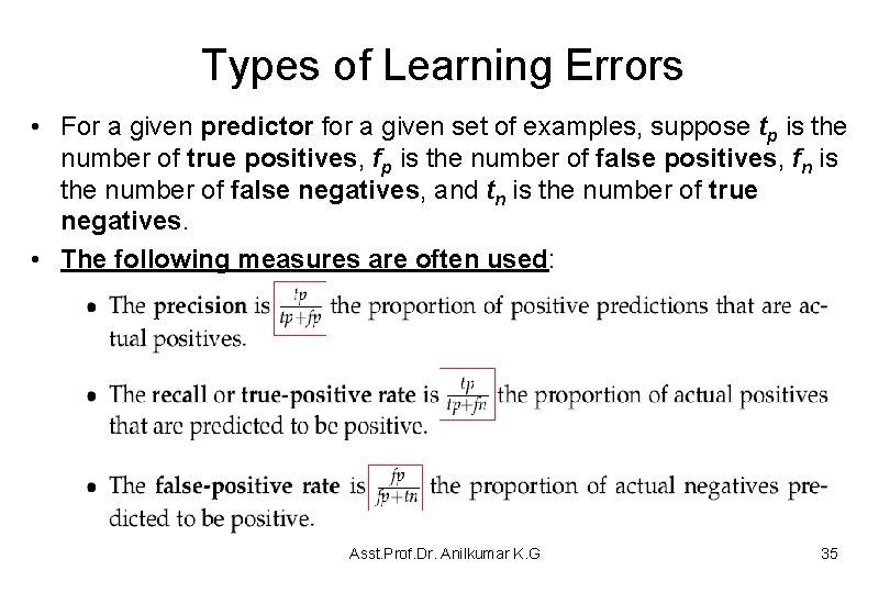
Types of Learning Errors • For a given predictor for a given set of examples, suppose tp is the number of true positives, fp is the number of false positives, fn is the number of false negatives, and tn is the number of true negatives. • The following measures are often used: Asst. Prof. Dr. Anilkumar K. G 35
Types of Learning Errors • An agent should try to maximize precision and recall and to minimize the false-positive rate and false-negative rate – however, these goals are incompatible. • An agent can maximize precision and minimize the falsepositive rate by only making positive predictions it is sure about. – However, this choice worsens recall. • To maximize recall, an agent can be risky in making predictions, which makes precision smaller and the falsepositive rate larger. Asst. Prof. Dr. Anilkumar K. G 36
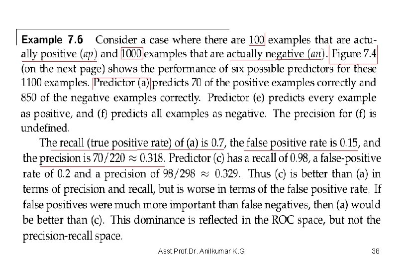
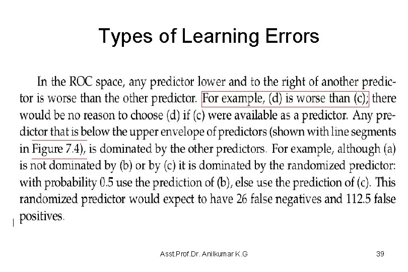
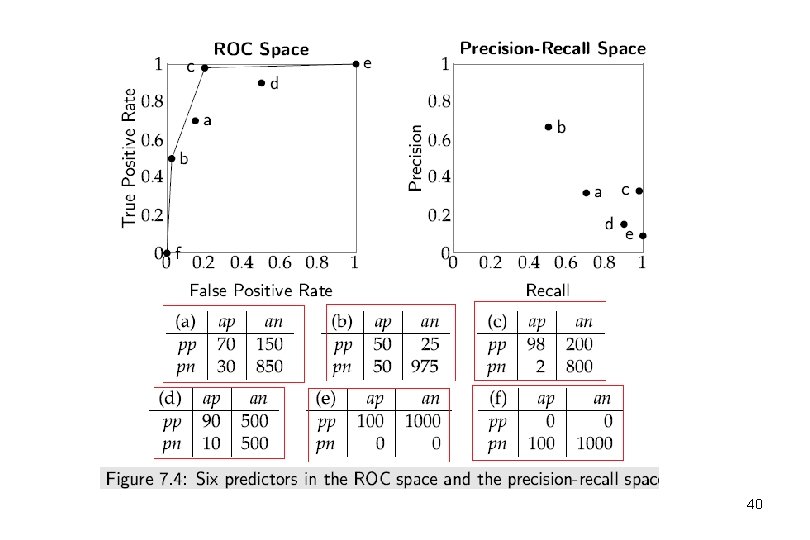
Types of Learning Errors • To compare predictors for a given set of examples, Receiver Operating Characteristic space (ROC space), plots the false-positive rate against the true-positive rate. – Each predictor for these examples becomes a point in the space. • A precision-recall space plots the precision against the recall. – Each of these approaches may be used to compare learning algorithms independently of the actual costs of the prediction errors. Asst. Prof. Dr. Anilkumar K. G 37
Asst. Prof. Dr. Anilkumar K. G 38
Types of Learning Errors Asst. Prof. Dr. Anilkumar K. G 39
Asst. Prof. Dr. Anilkumar K. G 40
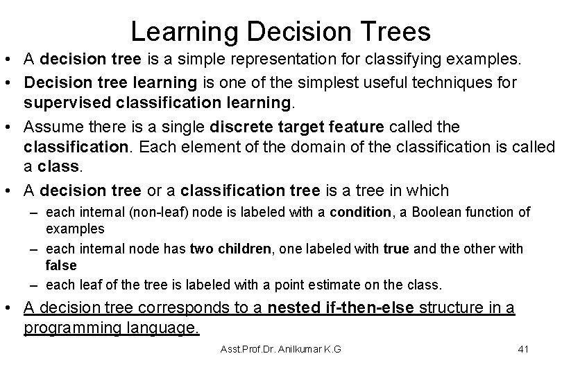
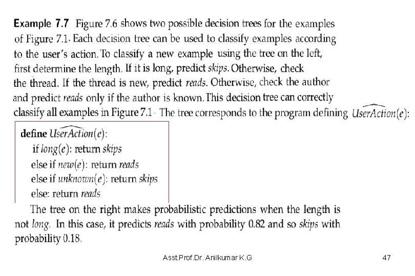
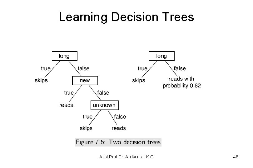
Learning Decision Trees • A decision tree is a simple representation for classifying examples. • Decision tree learning is one of the simplest useful techniques for supervised classification learning. • Assume there is a single discrete target feature called the classification. Each element of the domain of the classification is called a class. • A decision tree or a classification tree is a tree in which – each internal (non-leaf) node is labeled with a condition, a Boolean function of examples – each internal node has two children, one labeled with true and the other with false – each leaf of the tree is labeled with a point estimate on the class. • A decision tree corresponds to a nested if-then-else structure in a programming language. Asst. Prof. Dr. Anilkumar K. G 41
Learning Decision Trees • To classify an example, filter it down the tree, as follows: – Each condition encountered in the tree is evaluated and the arc corresponding to the result is followed. – When a leaf is reached, the classification corresponding to that leaf is returned. – A decision tree corresponds to a nested if-then-else structure in a programming language. Asst. Prof. Dr. Anilkumar K. G 42
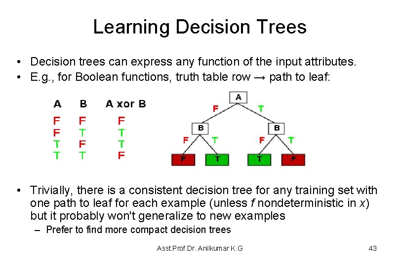
Learning Decision Trees • Decision trees can express any function of the input attributes. • E. g. , for Boolean functions, truth table row → path to leaf: • Trivially, there is a consistent decision tree for any training set with one path to leaf for each example (unless f nondeterministic in x) but it probably won't generalize to new examples – Prefer to find more compact decision trees Asst. Prof. Dr. Anilkumar K. G 43
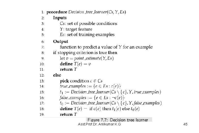
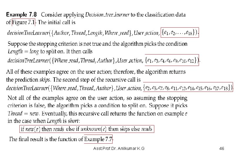
Learning Decision Trees • The algorithm Decision tree learner of Figure 7. 7 builds a decision tree from the top down as follows: – The input to the algorithm is a set of input conditions (Boolean functions of examples that use only input features), – target feature, and a set of training examples. – If the input features are Boolean, they can be used directly as the conditions. Asst. Prof. Dr. Anilkumar K. G 44
Asst. Prof. Dr. Anilkumar K. G 45
Asst. Prof. Dr. Anilkumar K. G 46
Asst. Prof. Dr. Anilkumar K. G 47
Learning Decision Trees Asst. Prof. Dr. Anilkumar K. G 48
Learning Decision Trees Asst. Prof. Dr. Anilkumar K. G 49
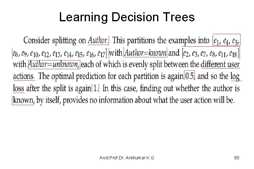
Learning Decision Trees Asst. Prof. Dr. Anilkumar K. G 50
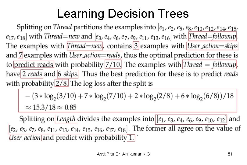
Learning Decision Trees Asst. Prof. Dr. Anilkumar K. G 51
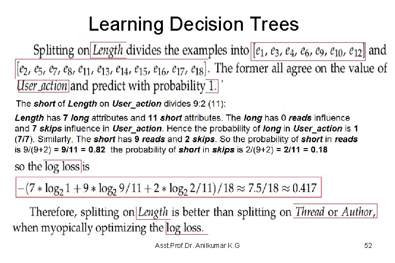
Learning Decision Trees Asst. Prof. Dr. Anilkumar K. G 52
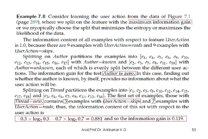
Asst. Prof. Dr. Anilkumar K. G 53
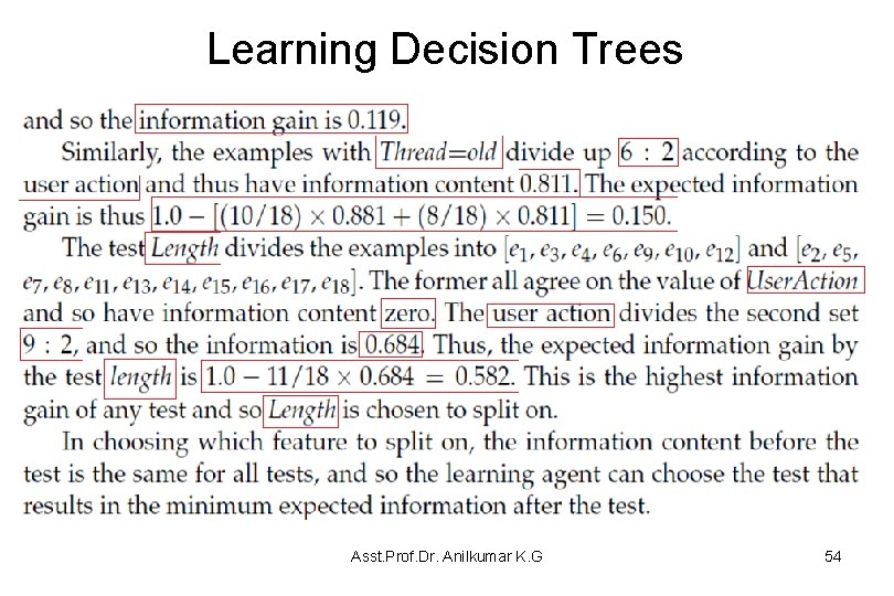
Learning Decision Trees Asst. Prof. Dr. Anilkumar K. G 54
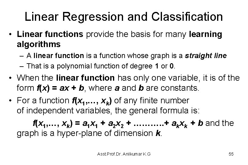
Linear Regression and Classification • Linear functions provide the basis for many learning algorithms – A linear function is a function whose graph is a straight line – That is a polynomial function of degree 1 or 0. • When the linear function has only one variable, it is of the form f(x) = ax + b, where a and b are constants. • For a function f(x 1, …, xk) of any finite number of independent variables, the general formula is: f(x 1, …, xk) = a 1 x 1 + a 2 x 2 + ………. . + akxk + b and the graph is a hyper-plane of dimension k. Asst. Prof. Dr. Anilkumar K. G 55
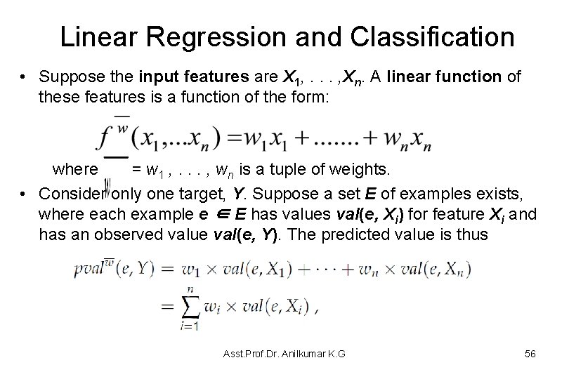
Linear Regression and Classification • Suppose the input features are X 1, . . . , Xn. A linear function of these features is a function of the form: where = w 1 , . . . , wn is a tuple of weights. • Consider only one target, Y. Suppose a set E of examples exists, where each example e ∈ E has values val(e, Xi) for feature Xi and has an observed value val(e, Y). The predicted value is thus Asst. Prof. Dr. Anilkumar K. G 56
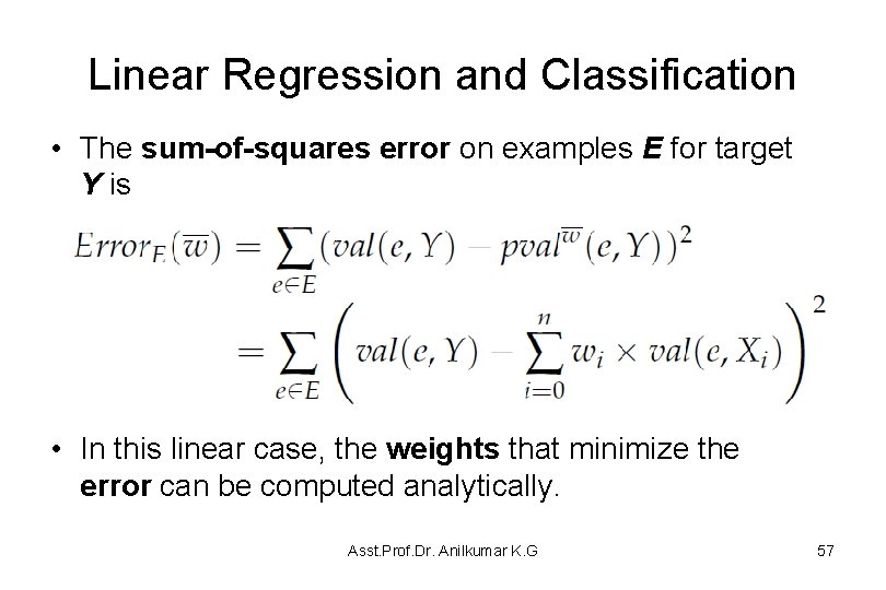
Linear Regression and Classification • The sum-of-squares error on examples E for target Y is • In this linear case, the weights that minimize the error can be computed analytically. Asst. Prof. Dr. Anilkumar K. G 57
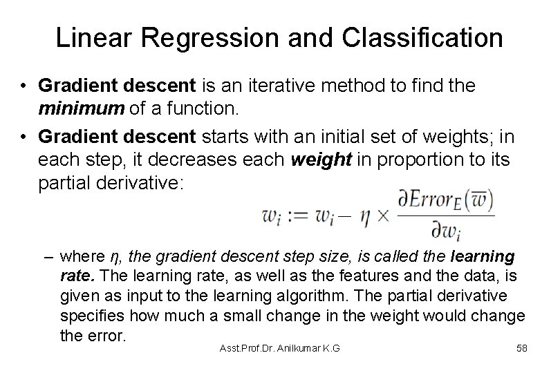
Linear Regression and Classification • Gradient descent is an iterative method to find the minimum of a function. • Gradient descent starts with an initial set of weights; in each step, it decreases each weight in proportion to its partial derivative: – where η, the gradient descent step size, is called the learning rate. The learning rate, as well as the features and the data, is given as input to the learning algorithm. The partial derivative specifies how much a small change in the weight would change the error. Asst. Prof. Dr. Anilkumar K. G 58
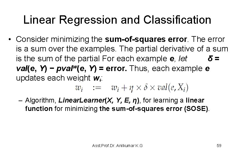
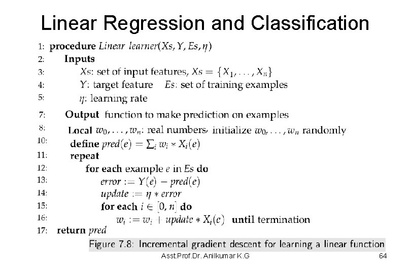
Linear Regression and Classification • Consider minimizing the sum-of-squares error. The error is a sum over the examples. The partial derivative of a sum is the sum of the partial For each example e, let δ= val(e, Y) − pvalw(e, Y) = error. Thus, each example e updates each weight wi: – Algorithm, Linear. Learner(X, Y, E, η), for learning a linear function for minimizing the sum-of-squares error (SOSE). Asst. Prof. Dr. Anilkumar K. G 59
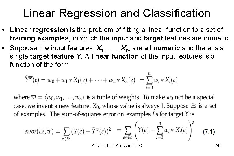
Linear Regression and Classification • Linear regression is the problem of fitting a linear function to a set of training examples, in which the input and target features are numeric. • Suppose the input features, X 1, . . . , Xn, are all numeric and there is a single target feature Y. A linear function of the input features is a function of the form Asst. Prof. Dr. Anilkumar K. G 60
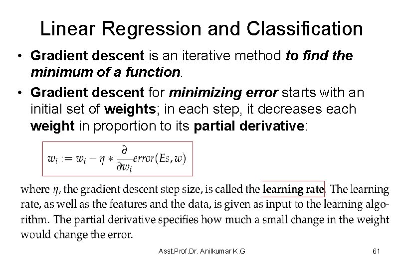
Linear Regression and Classification • Gradient descent is an iterative method to find the minimum of a function. • Gradient descent for minimizing error starts with an initial set of weights; in each step, it decreases each weight in proportion to its partial derivative: Asst. Prof. Dr. Anilkumar K. G 61
Linear Regression and Classification • The backpropagation keeps changing the neuron weights until there is greatest reduction in errors by an amount known as learning rate ( ). • Learning rate is a scalar parameter used to set the rate of adjustments to reduce the errors faster. • It is used to adjust weights and bias in backpropagation process. • More the learning rate, the faster the algorithm will reduce the errors and faster will be the training process. Asst. Prof. Dr. Anilkumar K. G 62
Linear Regression and Classification • Figure 7. 8 gives an algorithm, Linear learner(Xs, Y, Es, η), for learning the weights of a linear function that minimize the SOSE. • This algorithm returns a function that makes predictions on examples. • Termination is usually after some number of steps, when the error is small or when the changes get small. • Updating the weights after each example does not strictly implement gradient descent because the weights are changing between examples. • To implement gradient descent, we should save up all of the changes and update the weights after all of the examples have been processed. – The algorithm presented in Figure 7. 8 is called incremental gradient descent because the weights change while it iterates through the examples Asst. Prof. Dr. Anilkumar K. G 63
Linear Regression and Classification Asst. Prof. Dr. Anilkumar K. G 64
Linear Regression and Classification • The algorithm presented in Figure 7. 8 is called incremental gradient descent because the weights change while it iterates through the examples. • If the training examples are selected at random, this is called stochastic gradient descent. – These incremental methods have cheaper steps than gradient descent and so typically become more accurate more quickly when compared to saving all of the changes to the end of the examples. – However, it is not guaranteed that they will converge as individual examples can move the weights away from the minimum. Asst. Prof. Dr. Anilkumar K. G 65
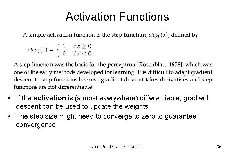
Activation Functions • If the activation is (almost everywhere) differentiable, gradient descent can be used to update the weights. • The step size might need to converge to zero to guarantee convergence. Asst. Prof. Dr. Anilkumar K. G 66
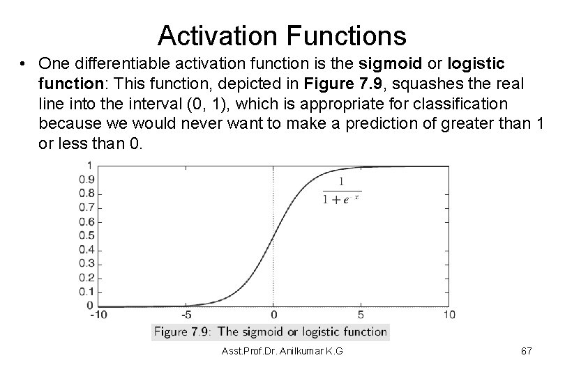
Activation Functions • One differentiable activation function is the sigmoid or logistic function: This function, depicted in Figure 7. 9, squashes the real line into the interval (0, 1), which is appropriate for classification because we would never want to make a prediction of greater than 1 or less than 0. Asst. Prof. Dr. Anilkumar K. G 67
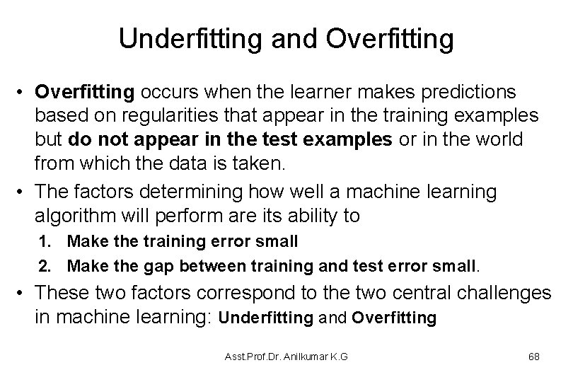
Underfitting and Overfitting • Overfitting occurs when the learner makes predictions based on regularities that appear in the training examples but do not appear in the test examples or in the world from which the data is taken. • The factors determining how well a machine learning algorithm will perform are its ability to 1. Make the training error small 2. Make the gap between training and test error small. • These two factors correspond to the two central challenges in machine learning: Underfitting and Overfitting Asst. Prof. Dr. Anilkumar K. G 68
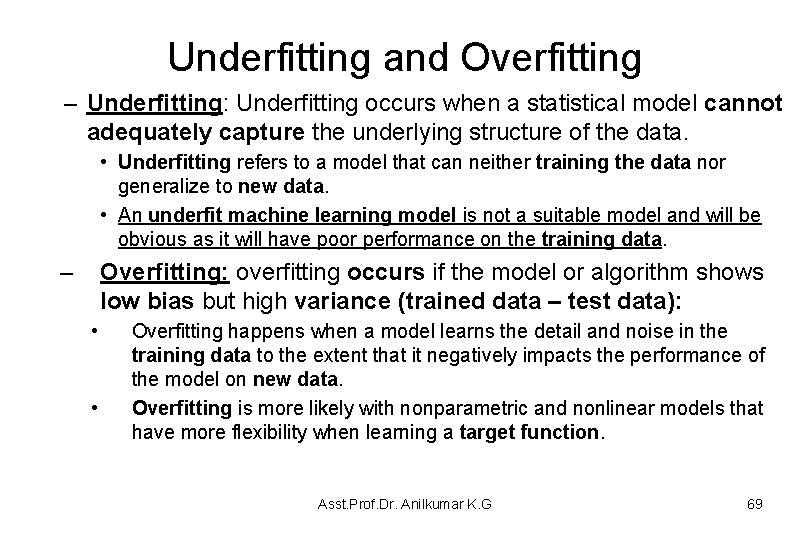
Underfitting and Overfitting – Underfitting: Underfitting occurs when a statistical model cannot adequately capture the underlying structure of the data. • Underfitting refers to a model that can neither training the data nor generalize to new data. • An underfit machine learning model is not a suitable model and will be obvious as it will have poor performance on the training data. – Overfitting: overfitting occurs if the model or algorithm shows low bias but high variance (trained data – test data): • • Overfitting happens when a model learns the detail and noise in the training data to the extent that it negatively impacts the performance of the model on new data. Overfitting is more likely with nonparametric and nonlinear models that have more flexibility when learning a target function. Asst. Prof. Dr. Anilkumar K. G 69
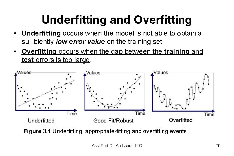
Underfitting and Overfitting • Underfitting occurs when the model is not able to obtain a su�ciently low error value on the training set. • Overfitting occurs when the gap between the training and test errors is too large. Figure 3. 1 Underfitting, appropriate-fitting and overfitting events Asst. Prof. Dr. Anilkumar K. G 70
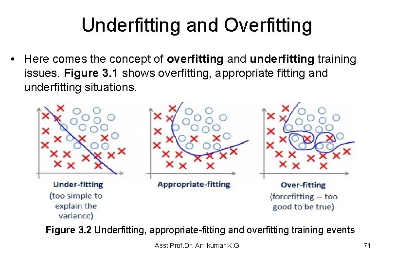
Underfitting and Overfitting • Here comes the concept of overfitting and underfitting training issues. Figure 3. 1 shows overfitting, appropriate fitting and underfitting situations. Figure 3. 2 Underfitting, appropriate-fitting and overfitting training events Asst. Prof. Dr. Anilkumar K. G 71
Underfitting and Overfitting – From figure 3. 2, by looking at the graph on the left side we can predict that the line does not cover all the points. Such model tend to cause underfitting of data, it also called High Bias. – Where as the graph on right side, shows the predicted line covers all the points in graph. – Such model are also responsible to predict poor result due to its complexity. Such model tend to cause overfitting of data (it is also called High Variance). • In such condition you can also think that it’s a good graph which cover all the points. • But that’s not actually true, the predicted line into the graph covers all points which are noise and outlier. Asst. Prof. Dr. Anilkumar K. G 72
Cross Validation • The idea of cross validation is to split the training dataset into two: – a dataset of examples to train with, – and a validation set. • The agent trains using the new training set. Prediction on the validation set is used to determine which model to use. • The idea of cross validation is to choose the representation in which the error of the validation set is a minimum. – In these cases, learning can continue until the error of the validation set starts to increase. Asst. Prof. Dr. Anilkumar K. G 73
Cross Validation • The validation set that is used as part of training is not the same as the test set. • The test set is used to evaluate how well the learning algorithm works as a whole. – It is cheating to use the test set as part of learning. • Remember that the aim is to predict examples that the agent has not seen. – The test set acts as a surrogate for these unseen examples, and so it cannot be used for training or validation. Asst. Prof. Dr. Anilkumar K. G 74
Cross Validation • One method, k-fold cross validation, is used to determine the best model complexity, such as the depth of a decision tree or the number of hidden units in a neural network. • The method of k-fold cross validation partitions the training dataset into k sets. • For each model complexity, the learner trains k times, each time using one of the sets as the validation set and the remaining sets as the training set. • It then selects the model complexity that has the smallest average error on the validation set (averaging over the k runs). • It can return the model with that complexity, trained on all of the data. Asst. Prof. Dr. Anilkumar K. G 75
- Slides: 75