Chapter 7 Simple Linear Regression for Forecasting Chapter

Chapter 7 Simple Linear Regression for Forecasting

Chapter 7: Simple Linear Regression for Forecasting 7. 1 Relationship between Variables: Correlation and Causation 7. 2 Fitting a Regression Line by Ordinary Least Squares (OLS) 7. 3 A Case Study on the Price of Gasoline 7. 4 How Good is the Fitted Line? 7. 5 The Statistical Framework for Regression 7. 6 Testing the Slope 7. 7 Forecasting Using Simple Linear Regression 7. 8 Forecasting Using Leading Indicators © 2017 Wessex Press, Inc. Principles of Business Forecasting 2 e (Ord, Fildes, Kourentzes) • Chapter 7: Simple Linear Regression for Forecasting 2

7. 1 Relationships between Variables: Correlation and Causation • In a causal model we are able to identify the known factors that determine future values of the dependent variable (denoted by Y), apart from the unknown random error. • Statistical correlation implies an association between two variables, but does not imply causality • Variables may be correlated because of a mutual connection to other variables. Question: The following pairs of variables are correlated. Is there a causal relationship? If so, which variable has a causal effect on the other? • • Height and Weight Knowledge of Statistics and Number of Cars Owned Advertising and Sales Down Jones Index and Gross Domestic Product © 2017 Wessex Press, Inc. Principles of Business Forecasting 2 e (Ord, Fildes, Kourentzes) • Chapter 7: Simple Linear Regression for Forecasting 3

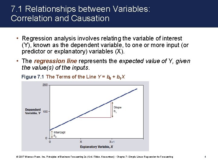
7. 1 Relationships between Variables: Correlation and Causation • Regression analysis involves relating the variable of interest (Y), known as the dependent variable, to one or more input (or predictor or explanatory) variables (X). • The regression line represents the expected value of Y, given the value(s) of the inputs. Figure 7. 1 The Terms of the Line Y = b 0 + b 1 X © 2017 Wessex Press, Inc. Principles of Business Forecasting 2 e (Ord, Fildes, Kourentzes) • Chapter 7: Simple Linear Regression for Forecasting 4

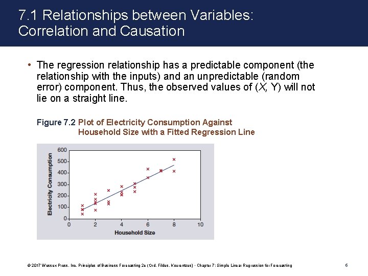
7. 1 Relationships between Variables: Correlation and Causation • The regression relationship has a predictable component (the relationship with the inputs) and an unpredictable (random error) component. Thus, the observed values of (X, Y) will not lie on a straight line. Figure 7. 2 Plot of Electricity Consumption Against Household Size with a Fitted Regression Line © 2017 Wessex Press, Inc. Principles of Business Forecasting 2 e (Ord, Fildes, Kourentzes) • Chapter 7: Simple Linear Regression for Forecasting 5

7. 1 Relationships between Variables: Correlation and Causation • Forecasting with a regression model may take one of several forms depending upon the information that is used as input to the forecasting process. –An ex ante, or unconditional, forecast uses only the information that would have been available at the time the forecast was made (i. e. , at the forecast origin). –An ex post, or conditional, forecast uses the actual values of the explanatory variables, even if these would not have been known at the time the forecast was made. –A what-if forecast uses assumed values of the explanatory variables to determine the potential outcomes of different policy alternatives or different possible futures. © 2017 Wessex Press, Inc. Principles of Business Forecasting 2 e (Ord, Fildes, Kourentzes) • Chapter 7: Simple Linear Regression for Forecasting 6

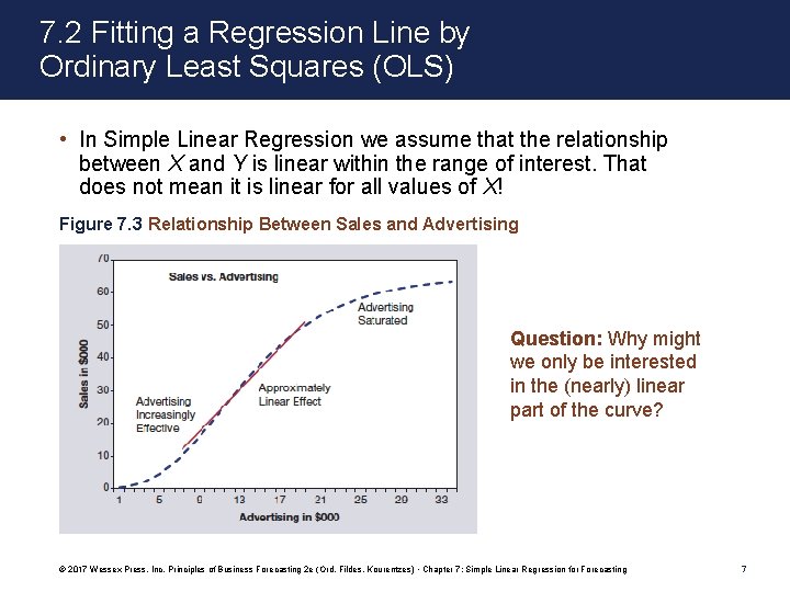
7. 2 Fitting a Regression Line by Ordinary Least Squares (OLS) • In Simple Linear Regression we assume that the relationship between X and Y is linear within the range of interest. That does not mean it is linear for all values of X! Figure 7. 3 Relationship Between Sales and Advertising Question: Why might we only be interested in the (nearly) linear part of the curve? © 2017 Wessex Press, Inc. Principles of Business Forecasting 2 e (Ord, Fildes, Kourentzes) • Chapter 7: Simple Linear Regression for Forecasting 7

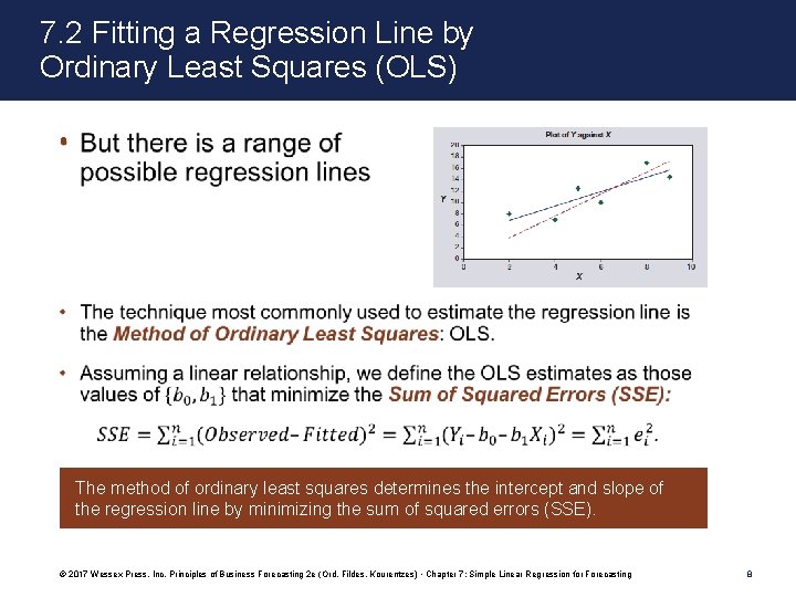
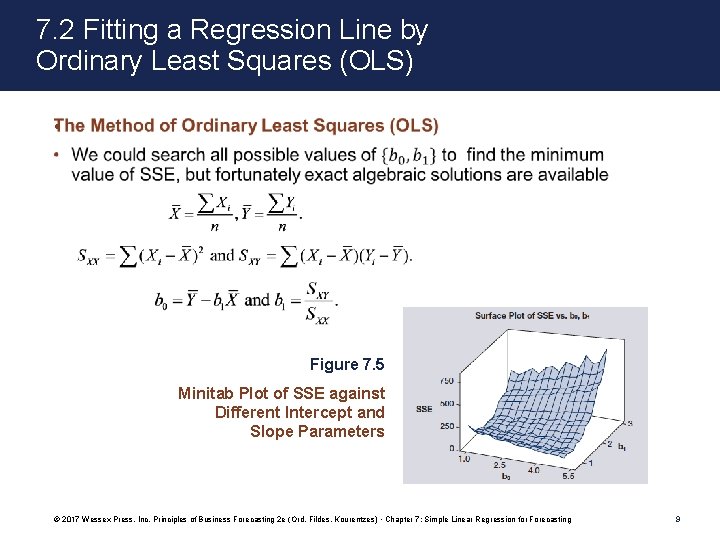
7. 2 Fitting a Regression Line by Ordinary Least Squares (OLS) • The method of ordinary least squares determines the intercept and slope of the regression line by minimizing the sum of squared errors (SSE). © 2017 Wessex Press, Inc. Principles of Business Forecasting 2 e (Ord, Fildes, Kourentzes) • Chapter 7: Simple Linear Regression for Forecasting 8

7. 2 Fitting a Regression Line by Ordinary Least Squares (OLS) • Figure 7. 5 Minitab Plot of SSE against Different Intercept and Slope Parameters © 2017 Wessex Press, Inc. Principles of Business Forecasting 2 e (Ord, Fildes, Kourentzes) • Chapter 7: Simple Linear Regression for Forecasting 9

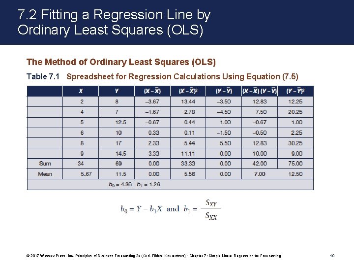
7. 2 Fitting a Regression Line by Ordinary Least Squares (OLS) The Method of Ordinary Least Squares (OLS) Table 7. 1 Spreadsheet for Regression Calculations Using Equation (7. 5) © 2017 Wessex Press, Inc. Principles of Business Forecasting 2 e (Ord, Fildes, Kourentzes) • Chapter 7: Simple Linear Regression for Forecasting 10

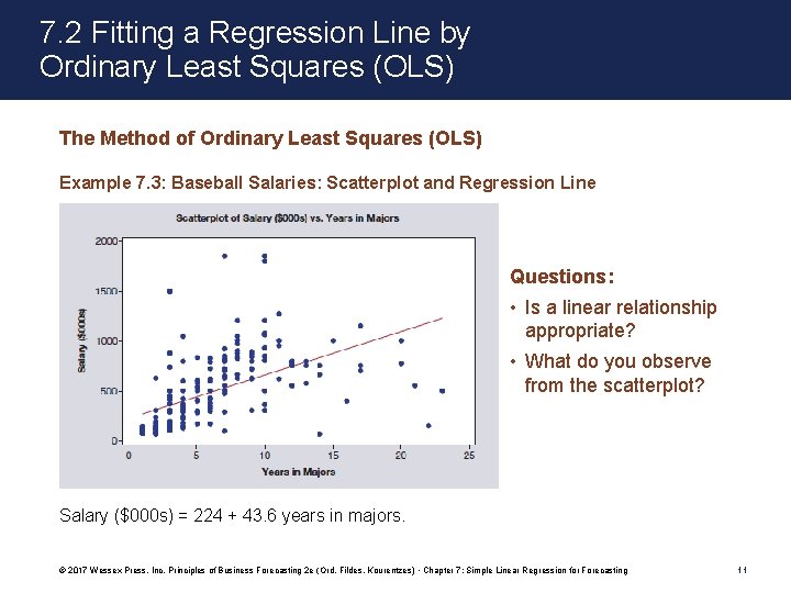
7. 2 Fitting a Regression Line by Ordinary Least Squares (OLS) The Method of Ordinary Least Squares (OLS) Example 7. 3: Baseball Salaries: Scatterplot and Regression Line Questions: • Is a linear relationship appropriate? • What do you observe from the scatterplot? Salary ($000 s) = 224 + 43. 6 years in majors. © 2017 Wessex Press, Inc. Principles of Business Forecasting 2 e (Ord, Fildes, Kourentzes) • Chapter 7: Simple Linear Regression for Forecasting 11

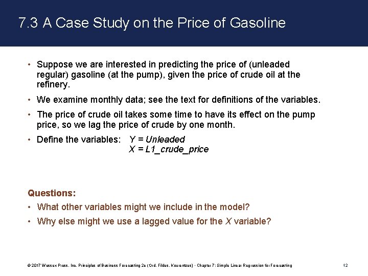
7. 3 A Case Study on the Price of Gasoline • Suppose we are interested in predicting the price of (unleaded regular) gasoline (at the pump), given the price of crude oil at the refinery. • We examine monthly data; see the text for definitions of the variables. • The price of crude oil takes some time to have its effect on the pump price, so we lag the price of crude by one month. • Define the variables: Y = Unleaded X = L 1_crude_price Questions: • What other variables might we include in the model? • Why else might we use a lagged value for the X variable? © 2017 Wessex Press, Inc. Principles of Business Forecasting 2 e (Ord, Fildes, Kourentzes) • Chapter 7: Simple Linear Regression for Forecasting 12

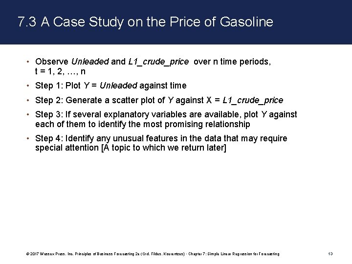
7. 3 A Case Study on the Price of Gasoline • Observe Unleaded and L 1_crude_price over n time periods, t = 1, 2, …, n • Step 1: Plot Y = Unleaded against time • Step 2: Generate a scatter plot of Y against X = L 1_crude_price • Step 3: If several explanatory variables are available, plot Y against each of them to identify the most promising relationship • Step 4: Identify any unusual features in the data that may require special attention [A topic to which we return later] © 2017 Wessex Press, Inc. Principles of Business Forecasting 2 e (Ord, Fildes, Kourentzes) • Chapter 7: Simple Linear Regression for Forecasting 13

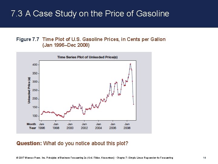
7. 3 A Case Study on the Price of Gasoline Figure 7. 7 Time Plot of U. S. Gasoline Prices, in Cents per Gallon (Jan 1996–Dec 2008) Question: What do you notice about this plot? © 2017 Wessex Press, Inc. Principles of Business Forecasting 2 e (Ord, Fildes, Kourentzes) • Chapter 7: Simple Linear Regression for Forecasting 14

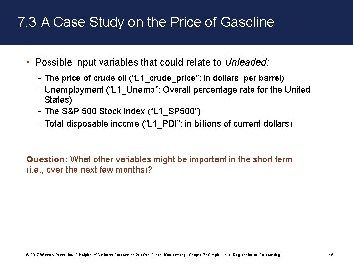
7. 3 A Case Study on the Price of Gasoline • Possible input variables that could relate to Unleaded: –The price of crude oil (“L 1_crude_price”; in dollars per barrel) –Unemployment (“L 1_Unemp”; Overall percentage rate for the United States) –The S&P 500 Stock Index (“L 1_SP 500”). –Total disposable income (“L 1_PDI”; in billions of current dollars) Question: What other variables might be important in the short term (i. e. , over the next few months)? © 2017 Wessex Press, Inc. Principles of Business Forecasting 2 e (Ord, Fildes, Kourentzes) • Chapter 7: Simple Linear Regression for Forecasting 15

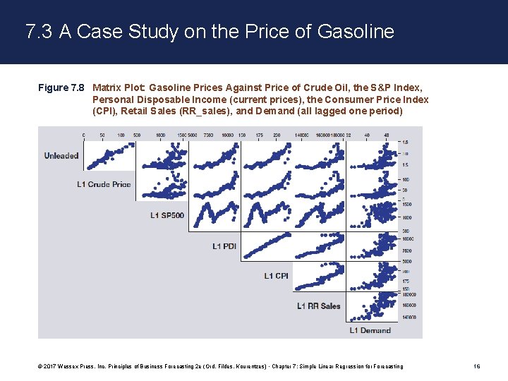
7. 3 A Case Study on the Price of Gasoline Figure 7. 8 Matrix Plot: Gasoline Prices Against Price of Crude Oil, the S&P Index, Personal Disposable Income (current prices), the Consumer Price Index (CPI), Retail Sales (RR_sales), and Demand (all lagged one period) © 2017 Wessex Press, Inc. Principles of Business Forecasting 2 e (Ord, Fildes, Kourentzes) • Chapter 7: Simple Linear Regression for Forecasting 16

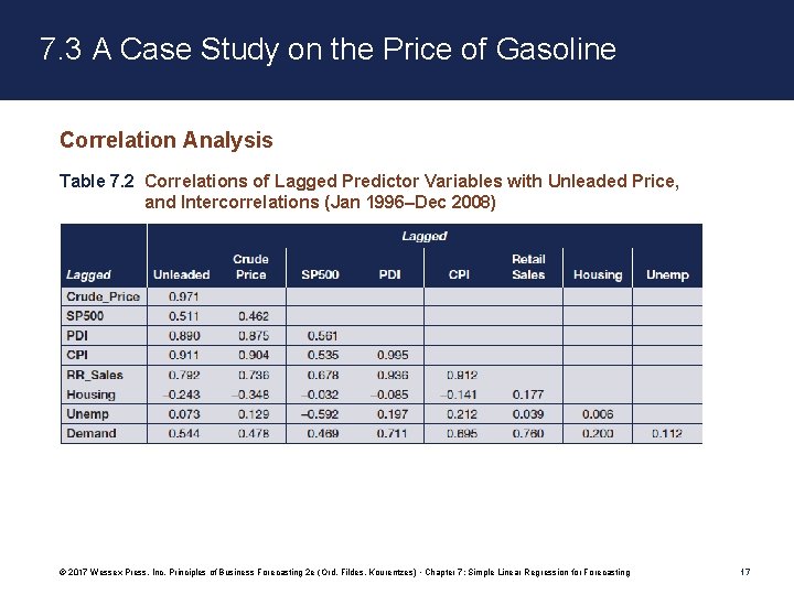
7. 3 A Case Study on the Price of Gasoline Correlation Analysis Table 7. 2 Correlations of Lagged Predictor Variables with Unleaded Price, and Intercorrelations (Jan 1996–Dec 2008) © 2017 Wessex Press, Inc. Principles of Business Forecasting 2 e (Ord, Fildes, Kourentzes) • Chapter 7: Simple Linear Regression for Forecasting 17

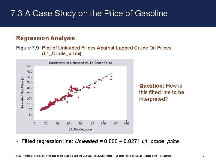
7. 3 A Case Study on the Price of Gasoline Regression Analysis Figure 7. 9 Plot of Unleaded Prices Against Lagged Crude Oil Prices (L 1_Crude_price) Question: How is this fitted line to be interpreted? • Fitted regression line: Unleaded = 0. 688 + 0. 0271 L 1_crude_price © 2017 Wessex Press, Inc. Principles of Business Forecasting 2 e (Ord, Fildes, Kourentzes) • Chapter 7: Simple Linear Regression for Forecasting 18

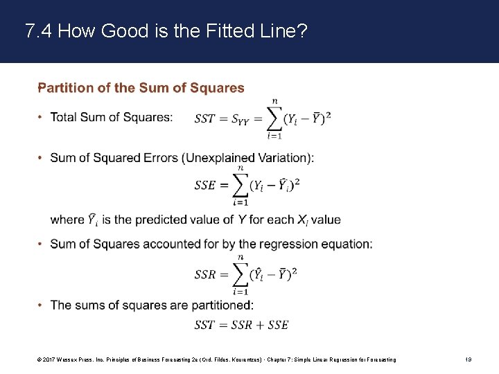
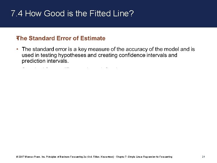
7. 4 How Good is the Fitted Line? • © 2017 Wessex Press, Inc. Principles of Business Forecasting 2 e (Ord, Fildes, Kourentzes) • Chapter 7: Simple Linear Regression for Forecasting 19

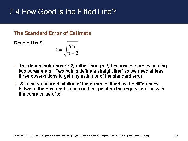
7. 4 How Good is the Fitted Line? The Standard Error of Estimate Denoted by S: • The denominator has (n-2) rather than (n-1) because we are estimating two parameters. “Two points define a straight line” so we need at least three observations to get any estimate of the standard error. • S is the standard deviation of the errors, defined as the differences between the observed values and the point on the regression line with the same value of X. © 2017 Wessex Press, Inc. Principles of Business Forecasting 2 e (Ord, Fildes, Kourentzes) • Chapter 7: Simple Linear Regression for Forecasting 20

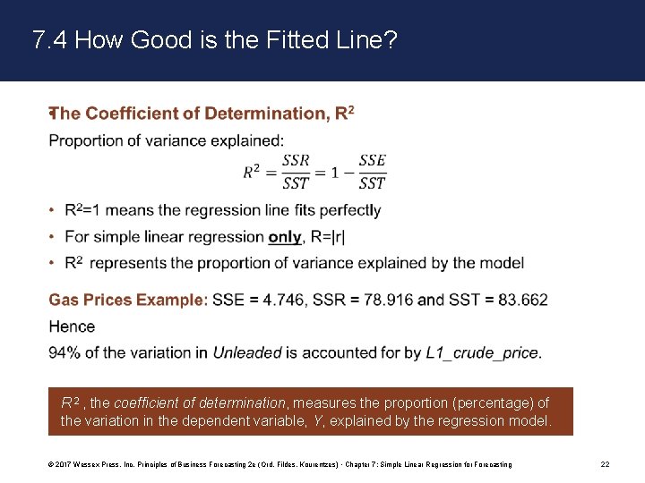
7. 4 How Good is the Fitted Line? • © 2017 Wessex Press, Inc. Principles of Business Forecasting 2 e (Ord, Fildes, Kourentzes) • Chapter 7: Simple Linear Regression for Forecasting 21

7. 4 How Good is the Fitted Line? • R 2 , the coefficient of determination, measures the proportion (percentage) of the variation in the dependent variable, Y, explained by the regression model. © 2017 Wessex Press, Inc. Principles of Business Forecasting 2 e (Ord, Fildes, Kourentzes) • Chapter 7: Simple Linear Regression for Forecasting 22

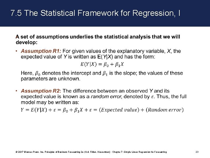
7. 5 The Statistical Framework for Regression, I • © 2017 Wessex Press, Inc. Principles of Business Forecasting 2 e (Ord, Fildes, Kourentzes) • Chapter 7: Simple Linear Regression for Forecasting 23

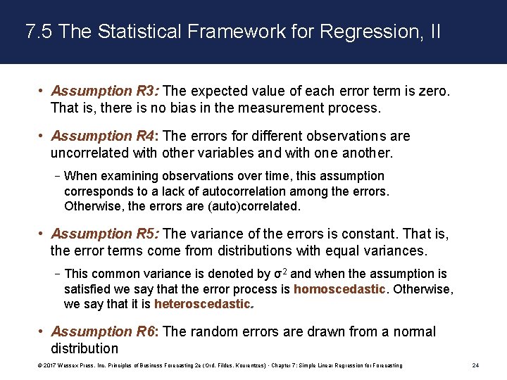
7. 5 The Statistical Framework for Regression, II • Assumption R 3: The expected value of each error term is zero. That is, there is no bias in the measurement process. • Assumption R 4: The errors for different observations are uncorrelated with other variables and with one another. –When examining observations over time, this assumption corresponds to a lack of autocorrelation among the errors. Otherwise, the errors are (auto)correlated. • Assumption R 5: The variance of the errors is constant. That is, the error terms come from distributions with equal variances. –This common variance is denoted by σ2 and when the assumption is satisfied we say that the error process is homoscedastic. Otherwise, we say that it is heteroscedastic. • Assumption R 6: The random errors are drawn from a normal distribution © 2017 Wessex Press, Inc. Principles of Business Forecasting 2 e (Ord, Fildes, Kourentzes) • Chapter 7: Simple Linear Regression for Forecasting 24

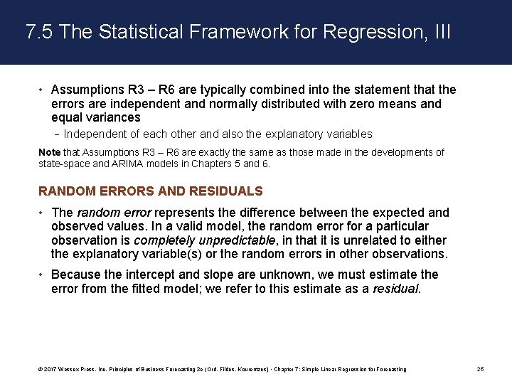
7. 5 The Statistical Framework for Regression, III • Assumptions R 3 – R 6 are typically combined into the statement that the errors are independent and normally distributed with zero means and equal variances – Independent of each other and also the explanatory variables Note that Assumptions R 3 – R 6 are exactly the same as those made in the developments of state-space and ARIMA models in Chapters 5 and 6. RANDOM ERRORS AND RESIDUALS • The random error represents the difference between the expected and observed values. In a valid model, the random error for a particular observation is completely unpredictable, in that it is unrelated to either the explanatory variable(s) or the random errors in other observations. • Because the intercept and slope are unknown, we must estimate the error from the fitted model; we refer to this estimate as a residual. © 2017 Wessex Press, Inc. Principles of Business Forecasting 2 e (Ord, Fildes, Kourentzes) • Chapter 7: Simple Linear Regression for Forecasting 25

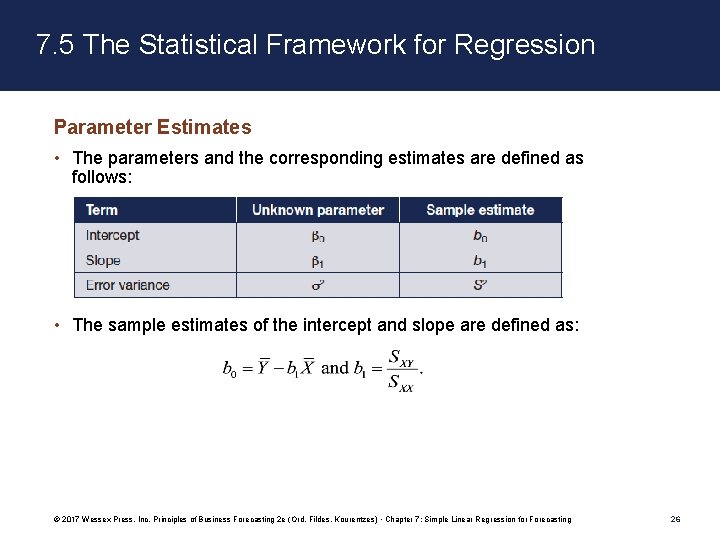
7. 5 The Statistical Framework for Regression Parameter Estimates • The parameters and the corresponding estimates are defined as follows: • The sample estimates of the intercept and slope are defined as: © 2017 Wessex Press, Inc. Principles of Business Forecasting 2 e (Ord, Fildes, Kourentzes) • Chapter 7: Simple Linear Regression for Forecasting 26

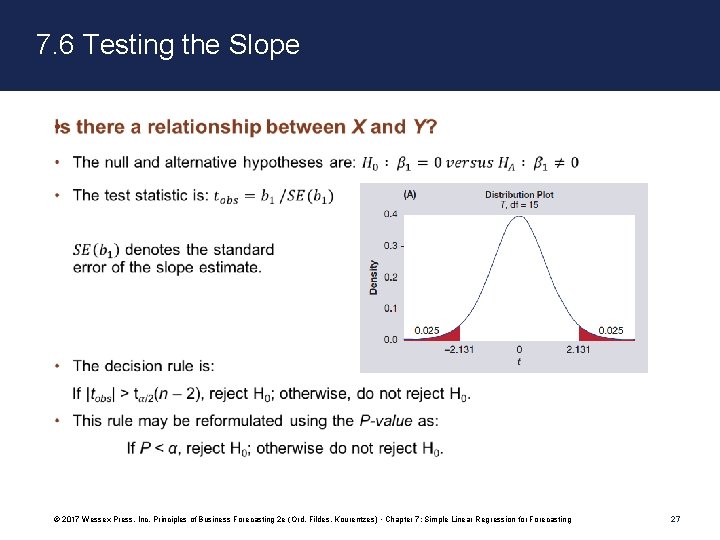
7. 6 Testing the Slope • © 2017 Wessex Press, Inc. Principles of Business Forecasting 2 e (Ord, Fildes, Kourentzes) • Chapter 7: Simple Linear Regression for Forecasting 27

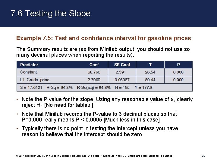
7. 6 Testing the Slope Example 7. 5: Test and confidence interval for gasoline prices The Summary results are (as from Minitab output; you should not use so many decimal places when reporting the results): • Note the P value for the slope: Using any reasonable value of α, clearly reject H 0 [No need for tables!] • Note that Minitab records the P-value to 3 decimal places so that P=0. 000 really means P < 0. 0005 [Much less in this case] • Typically there is no point in testing the intercept unless you have reason to believe that the intercept should be zero © 2017 Wessex Press, Inc. Principles of Business Forecasting 2 e (Ord, Fildes, Kourentzes) • Chapter 7: Simple Linear Regression for Forecasting 28

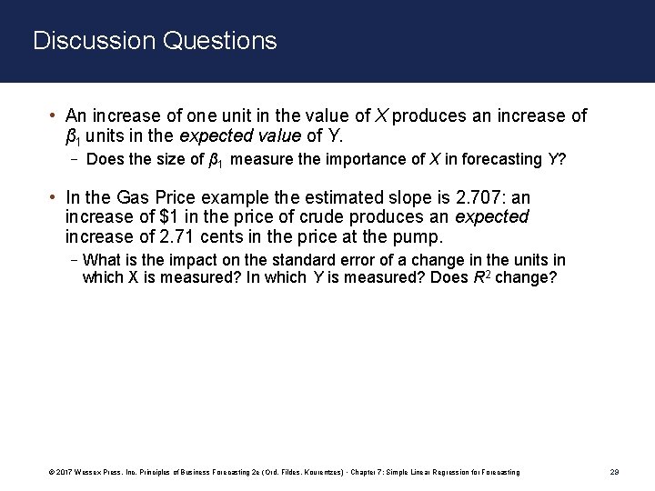
Discussion Questions • An increase of one unit in the value of X produces an increase of β 1 units in the expected value of Y. – Does the size of β 1 measure the importance of X in forecasting Y? • In the Gas Price example the estimated slope is 2. 707: an increase of $1 in the price of crude produces an expected increase of 2. 71 cents in the price at the pump. –What is the impact on the standard error of a change in the units in which X is measured? In which Y is measured? Does R 2 change? © 2017 Wessex Press, Inc. Principles of Business Forecasting 2 e (Ord, Fildes, Kourentzes) • Chapter 7: Simple Linear Regression for Forecasting 29

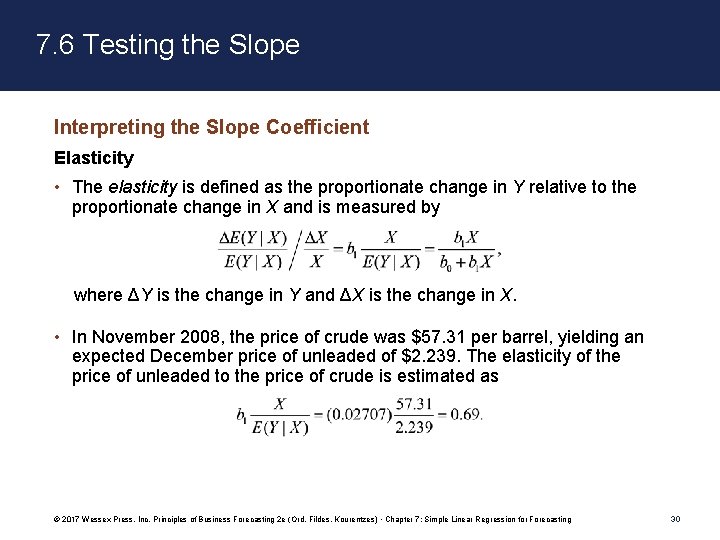
7. 6 Testing the Slope Interpreting the Slope Coefficient Elasticity • The elasticity is defined as the proportionate change in Y relative to the proportionate change in X and is measured by where ΔY is the change in Y and ΔX is the change in X. • In November 2008, the price of crude was $57. 31 per barrel, yielding an expected December price of unleaded of $2. 239. The elasticity of the price of unleaded to the price of crude is estimated as © 2017 Wessex Press, Inc. Principles of Business Forecasting 2 e (Ord, Fildes, Kourentzes) • Chapter 7: Simple Linear Regression for Forecasting 30

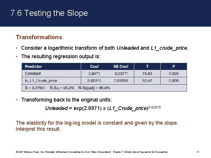
7. 6 Testing the Slope Transformations • Consider a logarithmic transform of both Unleaded and L 1_crude_price. • The resulting regression output is: • Transforming back to the original units: Unleaded = exp(2. 8971) x (L 1_Crude_price)0. 62815 The elasticity for the log-log model is constant and given by the slope. Interpret this result. © 2017 Wessex Press, Inc. Principles of Business Forecasting 2 e (Ord, Fildes, Kourentzes) • Chapter 7: Simple Linear Regression for Forecasting 31

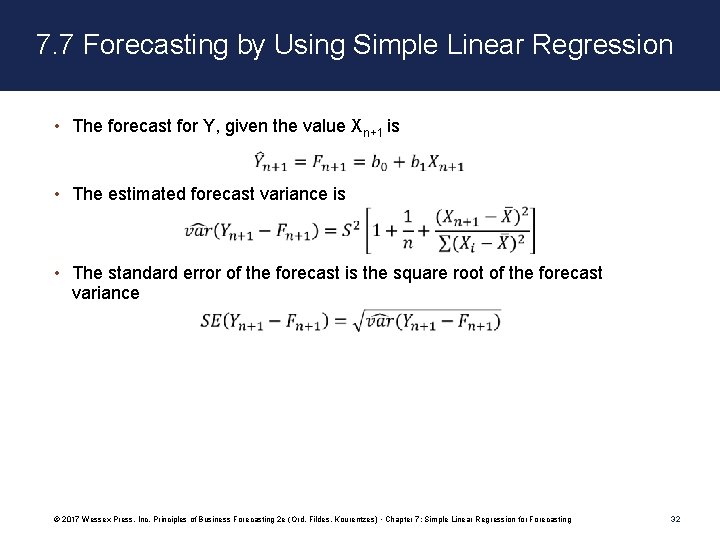
7. 7 Forecasting by Using Simple Linear Regression • The forecast for Y, given the value Xn+1 is • The estimated forecast variance is • The standard error of the forecast is the square root of the forecast variance © 2017 Wessex Press, Inc. Principles of Business Forecasting 2 e (Ord, Fildes, Kourentzes) • Chapter 7: Simple Linear Regression for Forecasting 32

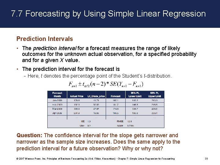
7. 7 Forecasting by Using Simple Linear Regression Prediction Intervals • The prediction interval for a forecast measures the range of likely outcomes for the unknown actual observation, for a specified probability and for a given X value. • The prediction interval for the forecast is – Here, t denotes the percentage point of the Student’s t-distribution. Question: The confidence interval for the slope gets narrower and narrower as the sample size increases. Does the same apply to the prediction interval for a future observation? Why or why not? © 2017 Wessex Press, Inc. Principles of Business Forecasting 2 e (Ord, Fildes, Kourentzes) • Chapter 7: Simple Linear Regression for Forecasting 33

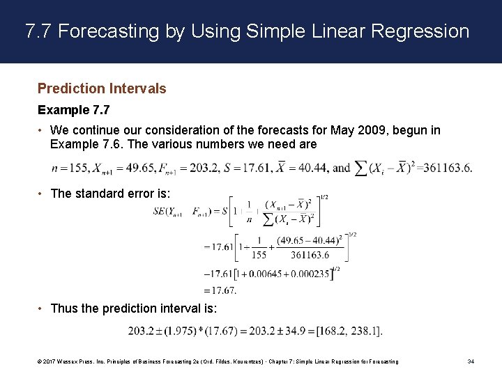
7. 7 Forecasting by Using Simple Linear Regression Prediction Intervals Example 7. 7 • We continue our consideration of the forecasts for May 2009, begun in Example 7. 6. The various numbers we need are • The standard error is: • Thus the prediction interval is: © 2017 Wessex Press, Inc. Principles of Business Forecasting 2 e (Ord, Fildes, Kourentzes) • Chapter 7: Simple Linear Regression for Forecasting 34

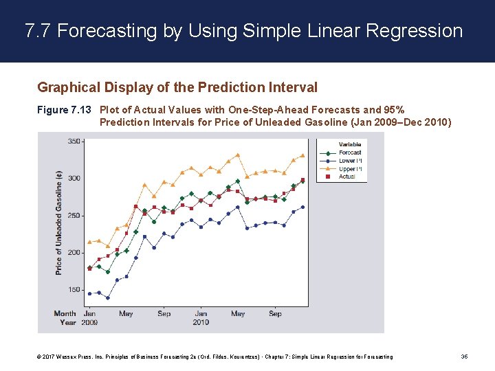
7. 7 Forecasting by Using Simple Linear Regression Graphical Display of the Prediction Interval Figure 7. 13 Plot of Actual Values with One-Step-Ahead Forecasts and 95% Prediction Intervals for Price of Unleaded Gasoline (Jan 2009–Dec 2010) © 2017 Wessex Press, Inc. Principles of Business Forecasting 2 e (Ord, Fildes, Kourentzes) • Chapter 7: Simple Linear Regression for Forecasting 35

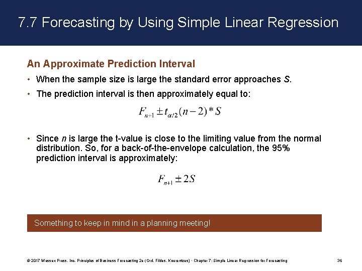
7. 7 Forecasting by Using Simple Linear Regression An Approximate Prediction Interval • When the sample size is large the standard error approaches S. • The prediction interval is then approximately equal to: • Since n is large the t-value is close to the limiting value from the normal distribution. So, for a back-of-the-envelope calculation, the 95% prediction interval is approximately: Something to keep in mind in a planning meeting! © 2017 Wessex Press, Inc. Principles of Business Forecasting 2 e (Ord, Fildes, Kourentzes) • Chapter 7: Simple Linear Regression for Forecasting 36

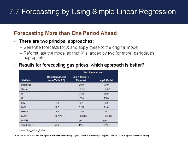
7. 7 Forecasting by Using Simple Linear Regression Forecasting More than One Period Ahead • There are two principal approaches: – Generate forecasts for X and apply these to the original model. – Reformulate the model so that X is lagged by two (or more) periods, as appropriate. • Results forecasting gas prices: which approach is better? © 2017 Wessex Press, Inc. Principles of Business Forecasting 2 e (Ord, Fildes, Kourentzes) • Chapter 7: Simple Linear Regression for Forecasting 37

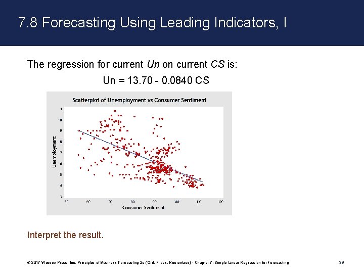
7. 8 Forecasting Using Leading Indicators, I • Consider the relationship between Unemployment [Un] and Consumer Sentiment [CS] –Monthly data available in Unemp_conconf_2. xlsx for January 1981 through December 2012; Un is a percentage and CS is measured on the scale (0, 100) © 2017 Wessex Press, Inc. Principles of Business Forecasting 2 e (Ord, Fildes, Kourentzes) • Chapter 7: Simple Linear Regression for Forecasting 38

7. 8 Forecasting Using Leading Indicators, I The regression for current Un on current CS is: Un = 13. 70 - 0. 0840 CS Interpret the result. © 2017 Wessex Press, Inc. Principles of Business Forecasting 2 e (Ord, Fildes, Kourentzes) • Chapter 7: Simple Linear Regression for Forecasting 39

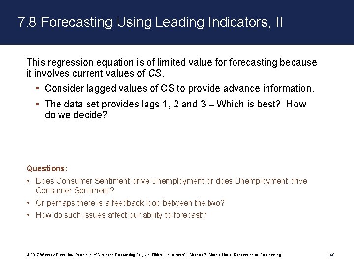
7. 8 Forecasting Using Leading Indicators, II This regression equation is of limited value forecasting because it involves current values of CS. • Consider lagged values of CS to provide advance information. • The data set provides lags 1, 2 and 3 – Which is best? How do we decide? Questions: • Does Consumer Sentiment drive Unemployment or does Unemployment drive Consumer Sentiment? • Or perhaps there is a feedback loop between the two? • How do such issues affect our ability to forecast? © 2017 Wessex Press, Inc. Principles of Business Forecasting 2 e (Ord, Fildes, Kourentzes) • Chapter 7: Simple Linear Regression for Forecasting 40

Take-Aways • Correlation does not imply causation; always try to select explanatory variables that have an economic (business or scientific) justification • A regression relationship may be linear within only a limited range of the observations, –we may not sensibly extrapolate outside that range without justification that the model still holds • It is good practice to check that the underlying assumptions are at least approximately valid. © 2017 Wessex Press, Inc. Principles of Business Forecasting 2 e (Ord, Fildes, Kourentzes) • Chapter 7: Simple Linear Regression for Forecasting 41

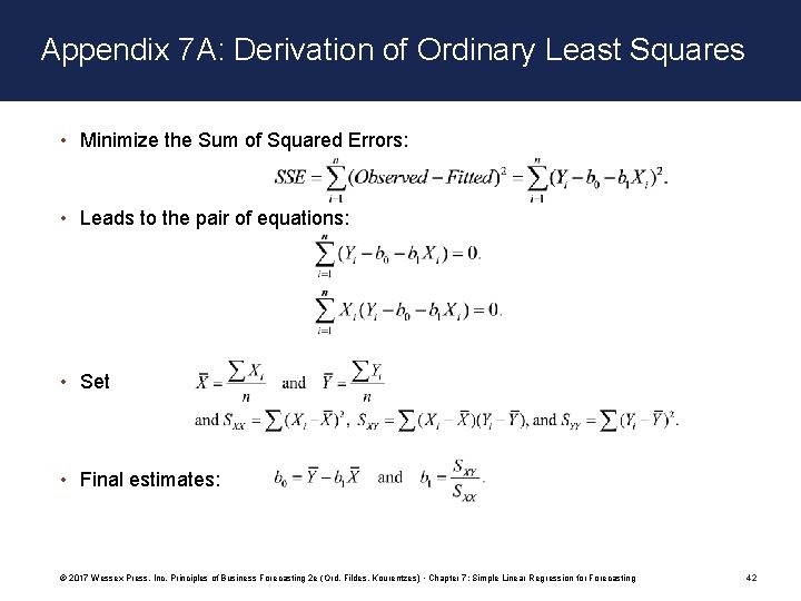
Appendix 7 A: Derivation of Ordinary Least Squares • Minimize the Sum of Squared Errors: • Leads to the pair of equations: • Set • Final estimates: © 2017 Wessex Press, Inc. Principles of Business Forecasting 2 e (Ord, Fildes, Kourentzes) • Chapter 7: Simple Linear Regression for Forecasting 42

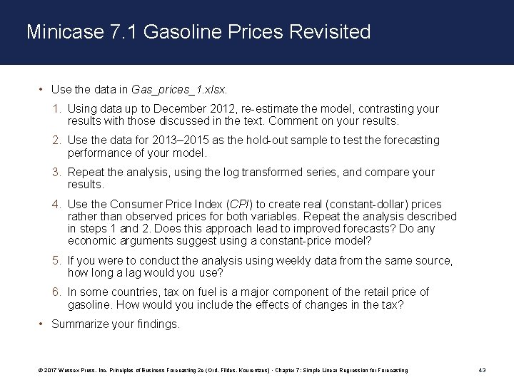
Minicase 7. 1 Gasoline Prices Revisited • Use the data in Gas_prices_1. xlsx. 1. Using data up to December 2012, re-estimate the model, contrasting your results with those discussed in the text. Comment on your results. 2. Use the data for 2013– 2015 as the hold-out sample to test the forecasting performance of your model. 3. Repeat the analysis, using the log transformed series, and compare your results. 4. Use the Consumer Price Index (CPI) to create real (constant-dollar) prices rather than observed prices for both variables. Repeat the analysis described in steps 1 and 2. Does this approach lead to improved forecasts? Do any economic arguments suggest using a constant-price model? 5. If you were to conduct the analysis using weekly data from the same source, how long a lag would you use? 6. In some countries, tax on fuel is a major component of the retail price of gasoline. How would you include the effects of changes in the tax? • Summarize your findings. © 2017 Wessex Press, Inc. Principles of Business Forecasting 2 e (Ord, Fildes, Kourentzes) • Chapter 7: Simple Linear Regression for Forecasting 43

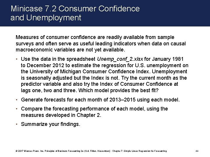
Minicase 7. 2 Consumer Confidence and Unemployment Measures of consumer confidence are readily available from sample surveys and often serve as useful leading indicators when data on causal macroeconomic variables are not yet available. • Use the data in the spreadsheet Unemp_conf_2. xlsx for January 1981 to December 2012 to estimate the regression for U. S. unemployment on the University of Michigan Consumer Confidence Index. Unemployment is seasonally adjusted but the Index is not. Try the current month as the predictor variable and also try the Index of Consumer Confidence at lags one, two and three. Which model provides the best fit? • Generate forecasts for each month of 2013– 2015 using each model. • Compare the forecasting performance of each model, using the measures developed in Chapter 2. • Summarize your findings. © 2017 Wessex Press, Inc. Principles of Business Forecasting 2 e (Ord, Fildes, Kourentzes) • Chapter 7: Simple Linear Regression for Forecasting 44

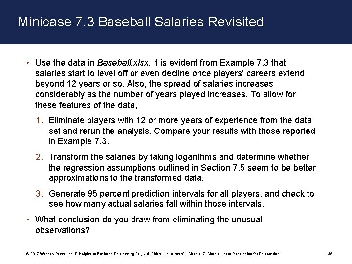
Minicase 7. 3 Baseball Salaries Revisited • Use the data in Baseball. xlsx. It is evident from Example 7. 3 that salaries start to level off or even decline once players’ careers extend beyond 12 years or so. Also, the spread of salaries increases considerably as the number of years played increases. To allow for these features of the data, 1. Eliminate players with 12 or more years of experience from the data set and rerun the analysis. Compare your results with those reported in Example 7. 3. 2. Transform the salaries by taking logarithms and determine whether the regression assumptions outlined in Section 7. 5 seem to be better approximations to the transformed data. 3. Generate 95 percent prediction intervals for all players, and check to see how many actual salaries fall within those intervals. • What conclusion do you draw from eliminating the unusual observations? © 2017 Wessex Press, Inc. Principles of Business Forecasting 2 e (Ord, Fildes, Kourentzes) • Chapter 7: Simple Linear Regression for Forecasting 45