Chapter 7 Sampling Distributions Section 7 1 How

Sampling Distribution App p Interactive Web p Explore statistical concepts in an interactive way. The following apps have graphs that update with clicks on buttons or sliders. Each explores a different statistical topic and allows results to be saved. Click on a picture to start the corresponding app. p http: //www. artofstat. com/webapps. html p Sampling Distribution of the Sample Proportion p https: //istats. shinyapps. io/Samp. Dist_Prop/ p Sampling Distribution of the Sample Mean p https: //istats. shinyapps. io/sampdist_cont/

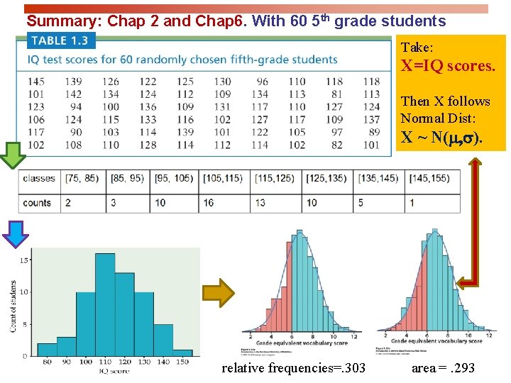
Summary: Chap 2 and Chap 6. With 60 5 th grade students Take: X=IQ scores. Then X follows Normal Dist: X ~ N(m, s). relative frequencies=. 303 area =. 293

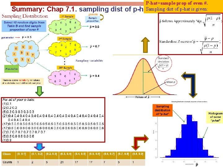
Summary: Chap 7. 1. sampling dist of P-hat=sample prop of even #. Sampling dist of p-hat is given: p-hat

Summary: Chap 7. 2. sampling dist of X-bar=sample mean. X-bar. Sampling dist of X-bar is given:

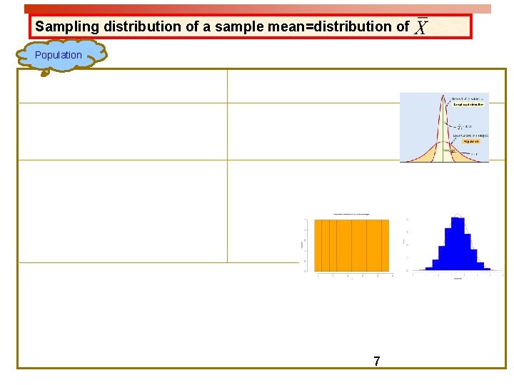
Chap 6: Distribution of X: Let X=height or height. X ~ N(m, s) Q: To find Probability with common three steps: Step 1. Standardize; That is, to find Z-score; Step 2: Draw N(0, 1) and shade; Step 3: Find: Prob=Area =NCDF(low, high, 0, 1) Chap 7. 1: Sampling dist. of sample Prop = Distribution of N(0, 1) Chap 7. 2: Sampling dist. of sample Mean = Distribution of Standardized height (no units)

Sampling distribution of a sample mean=distribution of Population 7

Comparison of Distributions in Chap 2, Chap 6, & Chap 7

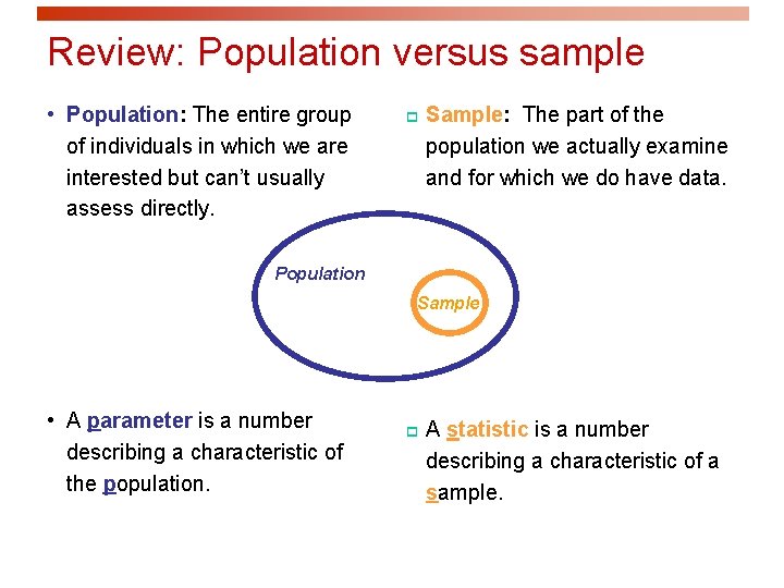
Review: Population versus sample • Population: The entire group of individuals in which we are interested but can’t usually assess directly. p Sample: The part of the population we actually examine and for which we do have data. Population Sample • A parameter is a number describing a characteristic of the population. p A statistic is a number describing a characteristic of a sample.

Objectives (chapter 7. 1) Sampling distribution of a sample proportion p Sampling distribution of sample proportion (p-hat) p For normally distributed populations p The central limit theorem Question: In high school, when doing Physics and Chemistry experiments, why do we need to repeat an experiment for multiple times? Then take an average as our final experiment result. It sounds to only waste our time, energy and materials on the repetition. Is it correct?

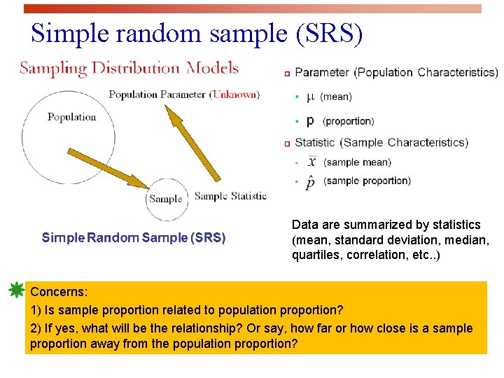
Simple random sample (SRS) Data are summarized by statistics (mean, standard deviation, median, quartiles, correlation, etc. . ) Concerns: 1) Is sample proportion related to population proportion? 2) If yes, what will be the relationship? Or say, how far or how close is a sample proportion away from the population proportion?

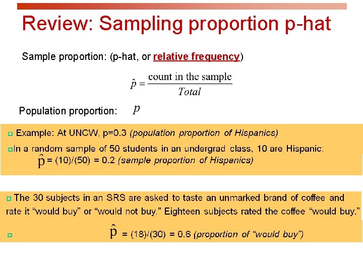
Review: Sampling proportion p-hat Sample proportion: (p-hat, or relative frequency) Population proportion:

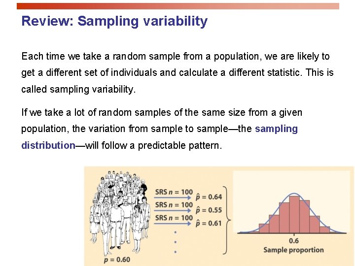
Review: Sampling variability Each time we take a random sample from a population, we are likely to get a different set of individuals and calculate a different statistic. This is called sampling variability. If we take a lot of random samples of the same size from a given population, the variation from sample to sample—the sampling distribution—will follow a predictable pattern.

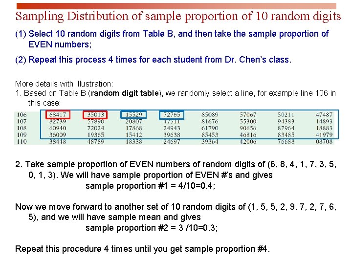
Sampling Distribution of sample proportion of 10 random digits (1) Select 10 random digits from Table B, and then take the sample proportion of EVEN numbers; (2) Repeat this process 4 times for each student from Dr. Chen’s class. More details with illustration: 1. Based on Table B (random digit table), we randomly select a line, for example line 106 in this case: 2. Take sample proportion of EVEN numbers of random digits of (6, 8, 4, 1, 7, 3, 5, 0, 1, 3). We will have sample proportion of EVEN #’s and gives sample proportion #1 = 4/10=0. 4; Now we move forward to another set of 10 random digits of (1, 5, 5, 2, 9, 7, 2, 7, 6, 5), and we will have sample mean and gives sample proportion #2 = 3 /10=0. 3; Repeat this procedure 4 times until you get sample proportion #4.

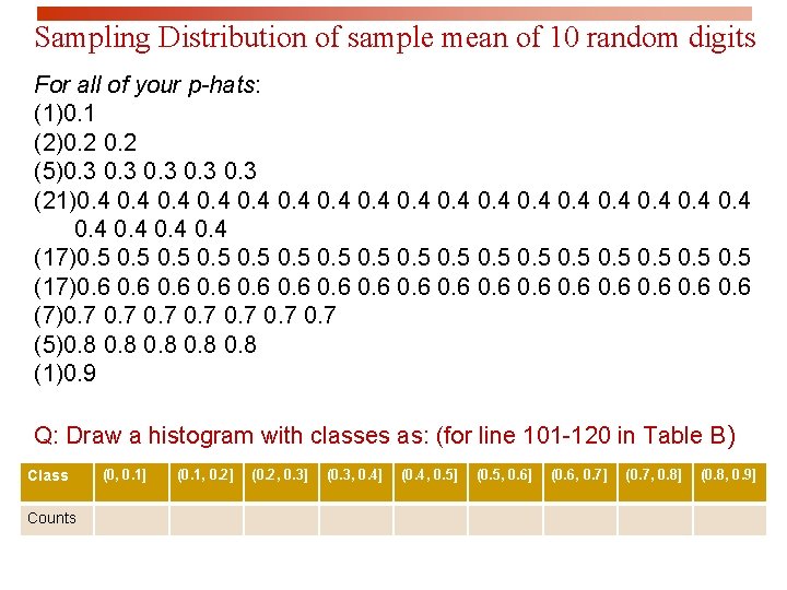
Sampling Distribution of sample mean of 10 random digits For all of your p-hats: (1)0. 1 (2)0. 2 (5)0. 3 0. 3 (21)0. 4 0. 4 (17)0. 5 0. 5 (17)0. 6 0. 6 (7)0. 7 0. 7 (5)0. 8 0. 8 (1)0. 9 Q: Draw a histogram with classes as: (for line 101 -120 in Table B) Class Counts (0, 0. 1] (0. 1, 0. 2] (0. 2, 0. 3] (0. 3, 0. 4] (0. 4, 0. 5] (0. 5, 0. 6] (0. 6, 0. 7] (0. 7, 0. 8] (0. 8, 0. 9]

Sampling Distribution of sample mean of 10 random digits Class (0, 0. 1] (0. 1, 0. 2] (0. 2, 0. 3] (0. 3, 0. 4] (0. 4, 0. 5] (0. 5, 0. 6] (0. 6, 0. 7] (0. 7, 0. 8] (0. 8, 0. 9] Counts 1 2 5 21 17 17 7 5 1 Q: Write a journal about how to get the sampling distribution of Sample proportion p-hat today, by answering the following questions: Sampling distribution of “p hat” Histogram of some sample proportion 1) How to obtain p-hat’s from Table B for each student? 2) How many p-hat’s did we have totally in the class? 3) How to make a histogram for p-hat? What is the name of the histogram? 4) What did the smooth curve represent? 5) For the smooth curve, what did the horizontal axis and vertical axis present?

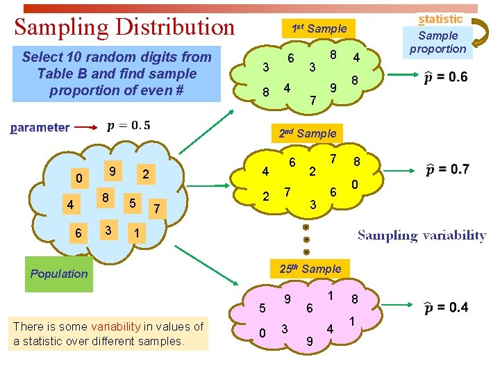
Sampling Distribution Select 10 random digits from Table B and find sample proportion of even # 1 st Sample 3 8 6 4 3 7 8 9 4 8 2 nd Sample 9 0 8 4 6 3 4 2 5 6 7 2 3 7 6 8 0 1 25 th Sample Population 5 There is some variability in values of a statistic over different samples. 0 9 3 6 9 1 4 8 1 Sample proportion

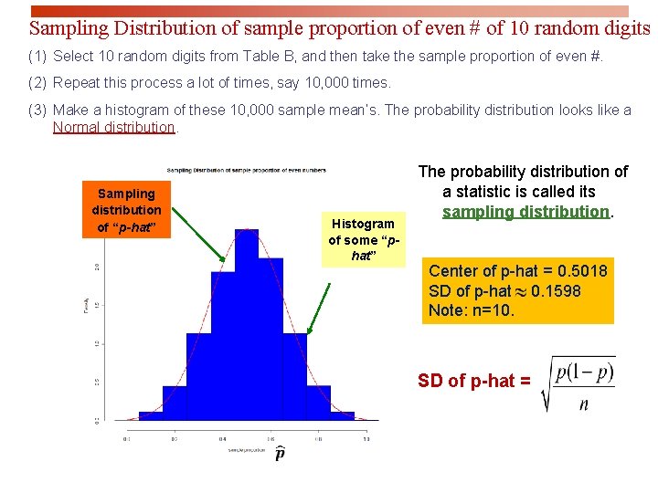
Sampling Distribution of sample proportion of even # of 10 random digits (1) Select 10 random digits from Table B, and then take the sample proportion of even #. (2) Repeat this process a lot of times, say 10, 000 times. (3) Make a histogram of these 10, 000 sample mean’s. The probability distribution looks like a Normal distribution. Sampling distribution of “p-hat” Histogram of some “phat” The probability distribution of a statistic is called its sampling distribution. Center of p-hat = 0. 5018 SD of p-hat = 0. 1598 Note: n=10. SD of p-hat =

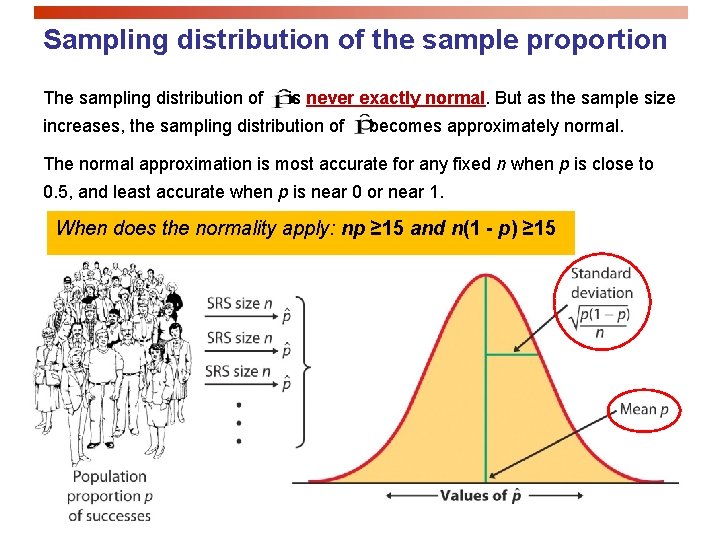
Sampling distribution of the sample proportion The sampling distribution of is never exactly normal. But as the sample size increases, the sampling distribution of becomes approximately normal. The normal approximation is most accurate for any fixed n when p is close to 0. 5, and least accurate when p is near 0 or near 1. When does the normality apply: np ≥ 15 and n(1 - p) ≥ 15

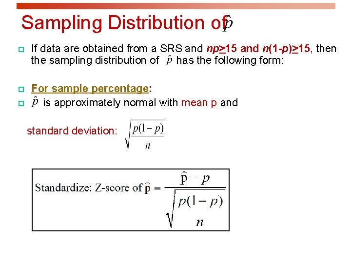
Sampling Distribution of p If data are obtained from a SRS and np>15 and n(1 -p)>15, then the sampling distribution of has the following form: p For sample percentage: is approximately normal with mean p and p standard deviation:

Sampling distribution of a sample Proportion = distribution of Note: data are obtained from a SRS and np>15 and 21 n(1 -p)>15.

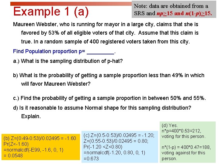
Example 1 (a) Note: data are obtained from a SRS and np>15 and n(1 -p)>15. Maureen Webster, who is running for mayor in a large city, claims that she is favored by 53% of all eligible voters of that city. Assume that this claim is true. In a random sample of 400 registered voters taken from this city. Find Population proportion p= _____. a. ) What is the sampling distribution of p-hat? b) What is the probability of getting a sample proportion less than 49% in which will favor Maureen Webster? c. ) Find the probability of getting a sample proportion in between 50% and 55%. d) Is it reasonable to assume Normal shape for this sampling distribution? Explain. (b) Z=(0. 49 -0. 53)/0. 02495 = -1. 60 Pr(Z<-1. 60) =normalcdf(-E 99, -1. 6, 0, 1) = 0. 0548 (c) Z=(0. 5 -0. 53)/0. 02495 = -1. 20; Z=(0. 55 -0. 53)/0. 02495 = 0. 80; Pr(-1. 20 <Z<0. 80) =normalcdf(-1. 20, 0. 80, 0, 1) =0. 673 (d) Yes. n*p=400*0. 53=212, voting for this person. n*(1 -p) = 400*0. 47=188, voting against for this person.

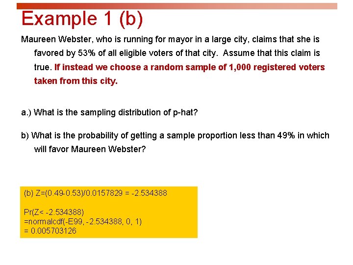
Example 1 (b) Maureen Webster, who is running for mayor in a large city, claims that she is favored by 53% of all eligible voters of that city. Assume that this claim is true. If instead we choose a random sample of 1, 000 registered voters taken from this city. a. ) What is the sampling distribution of p-hat? b) What is the probability of getting a sample proportion less than 49% in which will favor Maureen Webster? (b) Z=(0. 49 -0. 53)/0. 0157829 = -2. 534388 Pr(Z< -2. 534388) =normalcdf(-E 99, -2. 534388, 0, 1) = 0. 005703126

Example: Predicting Election Results Using Exit Polls How do we know if the sample proportion from the California exit poll is a good estimate, falling close to the population proportion? The total number of voters was over nine million, and the poll sampled a minuscule portion of them. This section introduces a type of probability distribution called the Sampling Distribution that helps us determine how close the sample proportion is to the population proportion. 24 Copyright © 2013, 2009, and 2007, Pearson Education, Inc.

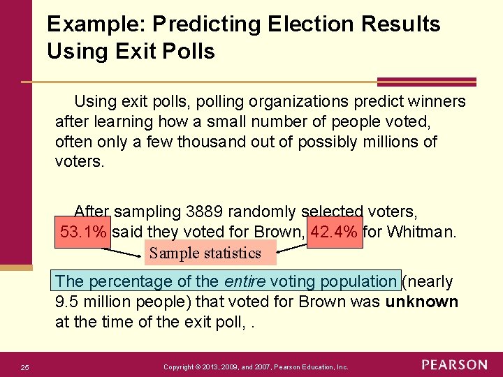
Example: Predicting Election Results Using Exit Polls Using exit polls, polling organizations predict winners after learning how a small number of people voted, often only a few thousand out of possibly millions of voters. After sampling 3889 randomly selected voters, 53. 1% said they voted for Brown, 42. 4% for Whitman. Sample statistics The percentage of the entire voting population (nearly 9. 5 million people) that voted for Brown was unknown at the time of the exit poll, . 25 Copyright © 2013, 2009, and 2007, Pearson Education, Inc.

Example: Predicting Election Results Using Exit Polls Let X = vote outcome, with: a) x = 1 for Jerry Brown; b) x = 0 for all other responses. The possible values of the random variable X (0 and 1) in the sample and how often these values occurred (0. 469 and 0. 531) give the data or sampling distribution for this one sample. The possible values of the random variable X (0 and 1) and how often these values occurred (0. 462 and 0. 538) give the population distribution. 26 Copyright © 2013, 2009, and 2007, Pearson Education, Inc.

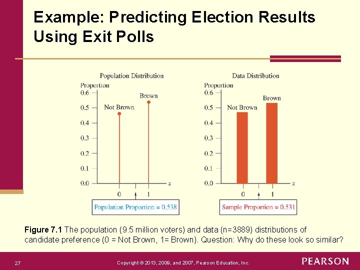
Example: Predicting Election Results Using Exit Polls Figure 7. 1 The population (9. 5 million voters) and data (n=3889) distributions of candidate preference (0 = Not Brown, 1= Brown). Question: Why do these look so similar? 27 Copyright © 2013, 2009, and 2007, Pearson Education, Inc.

Example: Predicting Election Results Using Exit Polls Sampling Distribution • The sampling distribution of a statistic is the probability distribution that specifies probabilities for the possible values the statistic can take. • The sampling distribution helps us determine how close to the population parameter a sample statistic is likely to fall. • A sampling distribution is merely a type of probability distribution. Rather than giving probabilities for an observation for an individual subject (as in a population or data distribution), it gives probabilities for the value of a statistic for a sample of subjects. Questions that we may solve: 1. How close can we expect a sample percentage to be to the population percentage? 2. How does the sample size influence our analysis? 28 Copyright © 2013, 2009, and 2007, Pearson Education, Inc.

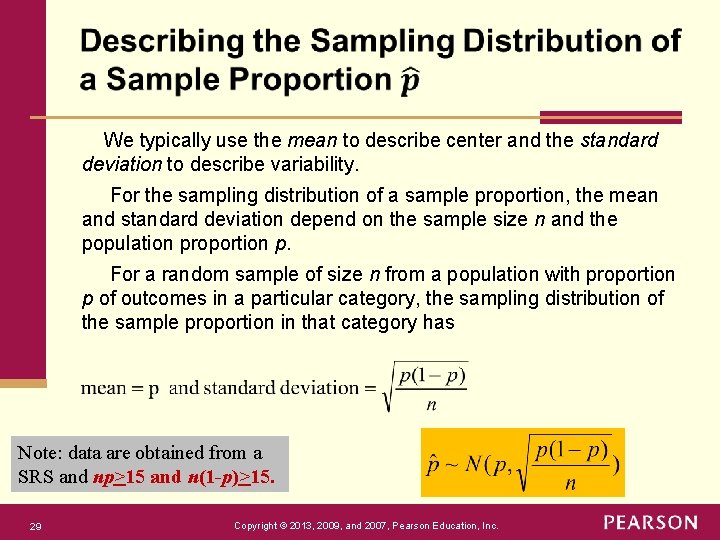
We typically use the mean to describe center and the standard deviation to describe variability. For the sampling distribution of a sample proportion, the mean and standard deviation depend on the sample size n and the population proportion p. For a random sample of size n from a population with proportion p of outcomes in a particular category, the sampling distribution of the sample proportion in that category has Note: data are obtained from a SRS and np>15 and n(1 -p)>15. 29 Copyright © 2013, 2009, and 2007, Pearson Education, Inc.

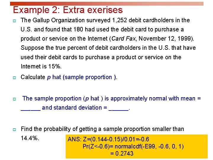
Example 2: Extra exerises p The Gallup Organization surveyed 1, 252 debit cardholders in the U. S. and found that 180 had used the debit card to purchase a product or service on the Internet (Card Fax, November 12, 1999). Suppose the true percent of debit cardholders in the U. S. that have used their debit cards to purchase a product or service on the Internet is 15%. p p Calculate p hat (sample proportion ). The sample proportion (p hat ) is approximately normal with mean = ______ and standard deviation = ______. p Find the probability of getting a sample proportion smaller than 14. 4%. ANS: Z=(0. 144 -0. 15)/0. 01=-0. 6 Pr(Z<-0. 6)= normalcdf(-E 99, -0. 6, 0, 1) = 0. 2743

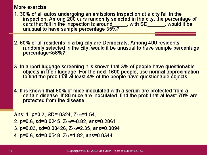
More exercise 1. 30% of all autos undergoing an emissions inspection at a city fail in the inspection. Among 200 cars randomly selected in the city, the percentage of cars that fail in the inspection is around_____, with SD______. would it be unusual to have sample percentage 35%? 2. 60% of all residents in a big city are Democrats. Among 400 residents randomly selected in the city, would it be unusual to have sample percentage<58%? 3. In airport luggage screening it is known that 3% of people have questionable objects in their luggage. For the next 1600 people, use normal approximation to find the prob that at least 4% of the people have questionable objects. 4. It is known that 60% of mice inoculated with a serum are protected from a certain disease. If 80 mice are inoculated, find the prob that at least 70% are protected from the disease. Ans: 1. p=0. 3, SD=. 0324, Z 0. 35=1. 54, 2. p=0. 6, sd=0. 0245, Z 0. 58=-0. 82, ans=0. 2061 3. p=0. 03, sd=0. 00426, Z 0. 04=2. 35, ans=0. 0094 4. p=0. 6, sd=0. 0548, Z 0. 7=1. 82, ans=0. 0344 31 Copyright © 2013, 2009, and 2007, Pearson Education, Inc.

Chapter 7 Sampling Distributions Section 7. 2 How Sample Means Vary Around the Population

Sampling Distribution App p Interactive Web p Explore statistical concepts in an interactive way. The following apps have graphs that update with clicks on buttons or sliders. Each explores a different statistical topic and allows results to be saved. Click on a picture to start the corresponding app. p http: //www. artofstat. com/webapps. html p Sampling Distribution of the Sample Proportion p https: //istats. shinyapps. io/Samp. Dist_Prop/ p Sampling Distribution of the Sample Mean p https: //istats. shinyapps. io/sampdist_cont/

Summary: Chap 2 and Chap 6. With 60 5 th grade students Take: X=IQ scores. Then X follows Normal Dist: X ~ N(m, s). relative frequencies=. 303 area =. 293

Summary: Chap 7. 1. sampling dist of P-hat=sample prop of even #. Sampling dist of p-hat is given: p-hat

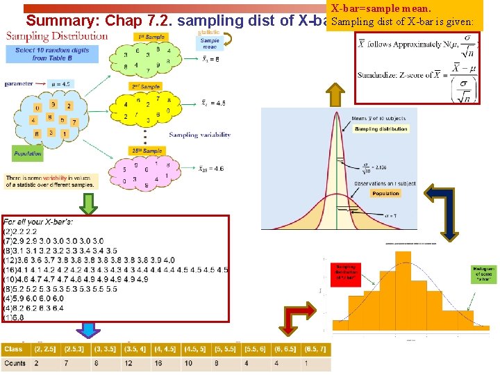
Summary: Chap 7. 2. sampling dist of X-bar=sample mean. X-bar. Sampling dist of X-bar is given:

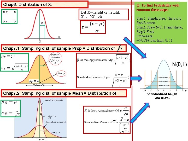
Chap 6: Distribution of X: Let X=height or height. X ~ N(m, s) Q: To find Probability with common three steps: Step 1. Standardize; That is, to find Z-score; Step 2: Draw N(0, 1) and shade; Step 3: Find: Prob=Area =NCDF(low, high, 0, 1) Chap 7. 1: Sampling dist. of sample Prop = Distribution of N(0, 1) Chap 7. 2: Sampling dist. of sample Mean = Distribution of Standardized height (no units)

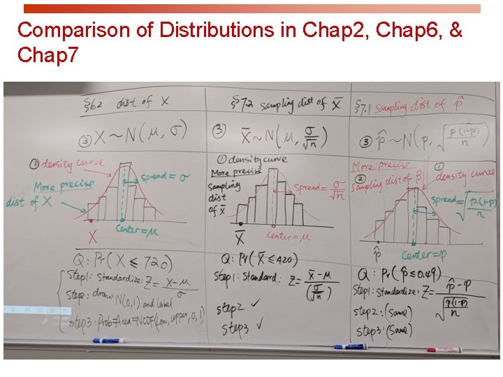
Comparison of Distributions in Chap 2, Chap 6, & Chap 7

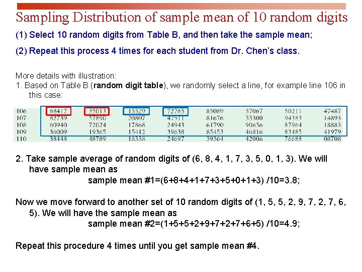
Sampling Distribution of sample mean of 10 random digits (1) Select 10 random digits from Table B, and then take the sample mean; (2) Repeat this process 4 times for each student from Dr. Chen’s class. More details with illustration: 1. Based on Table B (random digit table), we randomly select a line, for example line 106 in this case: 2. Take sample average of random digits of (6, 8, 4, 1, 7, 3, 5, 0, 1, 3). We will have sample mean as sample mean #1=(6+8+4+1+7+3+5+0+1+3) /10=3. 8; Now we move forward to another set of 10 random digits of (1, 5, 5, 2, 9, 7, 2, 7, 6, 5). We will have the sample mean as sample mean #2=(1+5+5+2+9+7+2+7+6+5) /10=4. 9; Repeat this procedure 4 times until you get sample mean #4.

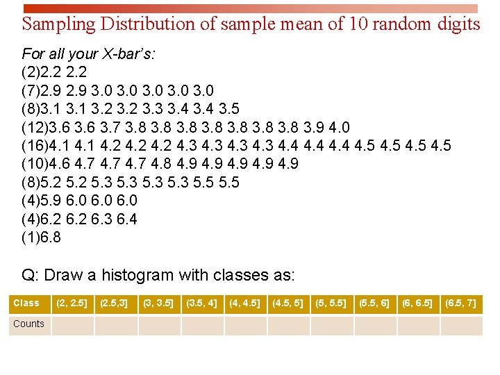
Sampling Distribution of sample mean of 10 random digits For all your X-bar’s: (2)2. 2 (7)2. 9 3. 0 3. 0 (8)3. 1 3. 2 3. 3 3. 4 3. 5 (12)3. 6 3. 7 3. 8 3. 9 4. 0 (16)4. 1 4. 2 4. 3 4. 4 4. 5 (10)4. 6 4. 7 4. 8 4. 9 4. 9 (8)5. 2 5. 3 5. 5 (4)5. 9 6. 0 (4)6. 2 6. 3 6. 4 (1)6. 8 Q: Draw a histogram with classes as: Class Counts (2, 2. 5] (2. 5, 3] (3, 3. 5] (3. 5, 4] (4, 4. 5] (4. 5, 5] (5, 5. 5] (5. 5, 6] (6, 6. 5] (6. 5, 7]

Sampling Distribution of sample mean of 10 random digits Class (2, 2. 5] (2. 5, 3] (3, 3. 5] (3. 5, 4] (4, 4. 5] (4. 5, 5] (5, 5. 5] (5. 5, 6] (6, 6. 5] (6. 5, 7] Counts 2 7 8 12 16 10 8 4 4 1 Sampling distribution of “x bar” Histogram of some “x bar” Q: Write a journal about how to get the sampling distribution of Sample mean X-bar today, by answering the following questions: 1) How to obtain X-bar’s, starting from Table B for each student? 2) How many X-bar’s did we have totally in the class? 3) How to make a histogram for X-bar? What is the name of the histogram? 4) What did the smooth curve represent? 5) For the smooth curve, what did the horizontal axis and vertical axis present?

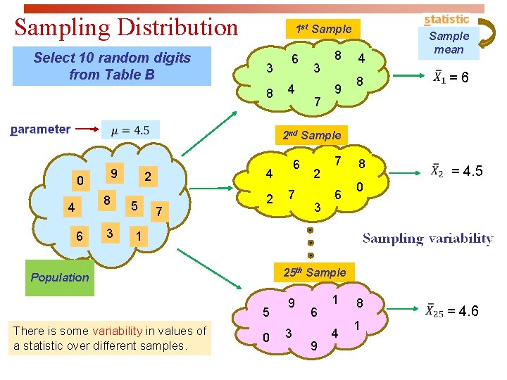
Sampling Distribution Select 10 random digits from Table B 1 st Sample 3 8 6 4 3 7 8 9 4 Sample mean 8 =6 8 = 4. 5 2 nd Sample 9 0 8 4 6 3 4 2 5 6 7 2 3 7 6 0 1 25 th Sample Population 5 There is some variability in values of a statistic over different samples. 0 9 3 6 9 1 4 8 1 = 4. 6

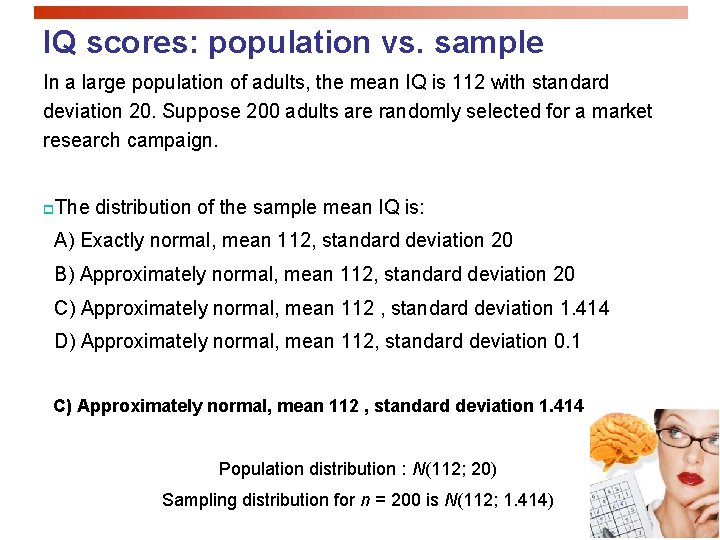
IQ scores: population vs. sample In a large population of adults, the mean IQ is 112 with standard deviation 20. Suppose 200 adults are randomly selected for a market research campaign. p. The distribution of the sample mean IQ is: A) Exactly normal, mean 112, standard deviation 20 B) Approximately normal, mean 112, standard deviation 20 C) Approximately normal, mean 112 , standard deviation 1. 414 D) Approximately normal, mean 112, standard deviation 0. 1 C) Approximately normal, mean 112 , standard deviation 1. 414 Population distribution : N(112; 20) Sampling distribution for n = 200 is N(112; 1. 414)

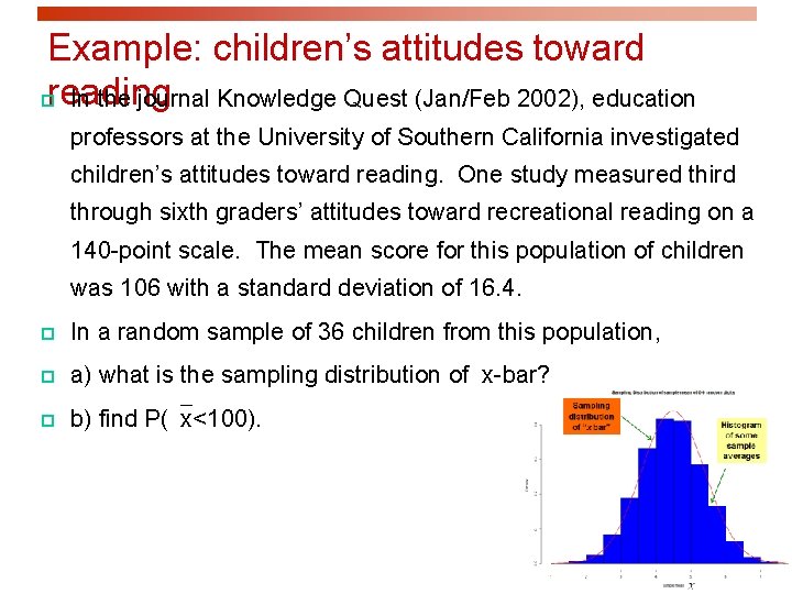
Example: children’s attitudes toward preading In the journal Knowledge Quest (Jan/Feb 2002), education professors at the University of Southern California investigated children’s attitudes toward reading. One study measured third through sixth graders’ attitudes toward recreational reading on a 140 -point scale. The mean score for this population of children was 106 with a standard deviation of 16. 4. p In a random sample of 36 children from this population, p a) what is the sampling distribution of x-bar? p b) find P( x<100).

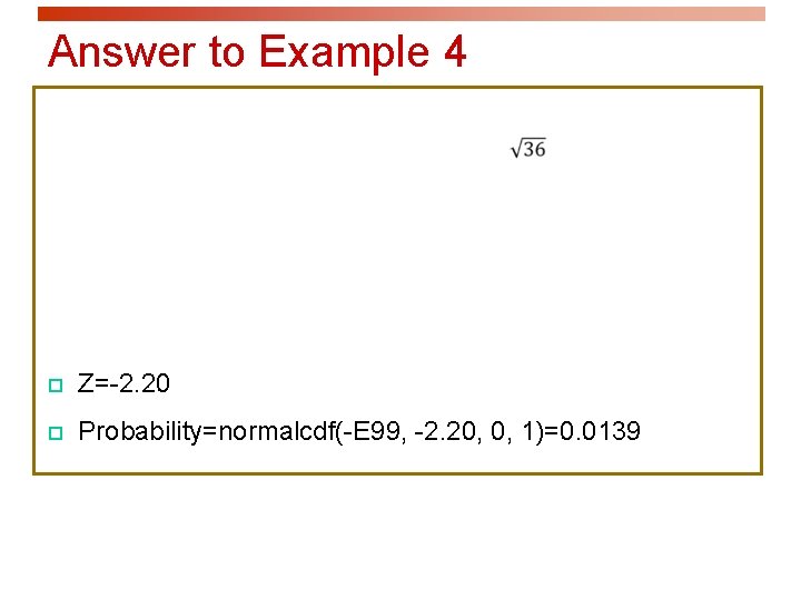
Answer to Example 4 p Z=-2. 20 p Probability=normalcdf(-E 99, -2. 20, 0, 1)=0. 0139

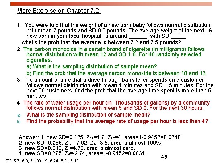
More Exercise on Chapter 7. 2: 1. You were told that the weight of a new born baby follows normal distribution with mean 7 pounds and SD 0. 5 pounds. The average weight of the next 16 new born in your local hospital is around ______, with SD _____. what’s the prob that the average is between 7. 2 and 7. 5 pounds? 2. The carbon monoxide in a certain brand of cigarette (in milligrams) follows normal distribution with mean 12 and SD 1. 8. For 40 randomly selected cigarettes, a) What is the sampling distribution of sample mean? b) Find the prob that the average carbon monoxide is between 10 and 13. 3. The amount of time that a drive-through bank teller spends on a customer follows normal distribution with mean 4 minutes and SD 1. 5 minutes. For the next 50 customers, find the prob that the average time spent is more than 5 minutes 4. The rate of water usage per hour (in Thousands of gallons) by a community follows normal distribution with mean 5 and SD 2. For the next 30 hours, a) What is the sampling distribution of sample mean? b) Find the probability that the average rate of usage per hour is less than 4? Answer: 1. new SD=0. 125, Z 7. 2=1. 6, Z 7. 5=4, area=1 -0. 9452=0. 0548 2. new SD=0. 285, Z 10=-7. 02, Z 13=3. 5, area is almost 100% 3. new SD=0. 212, Z 5=4. 72, area is almost zero. 4. new SD=0. 365, Z 4=-2. 74, area=1 -0. 9452=0. 0031. 46 EX: 5. 7, 5. 8, 5. 18(a-c), 5. 24, 5. 21, 5. 12

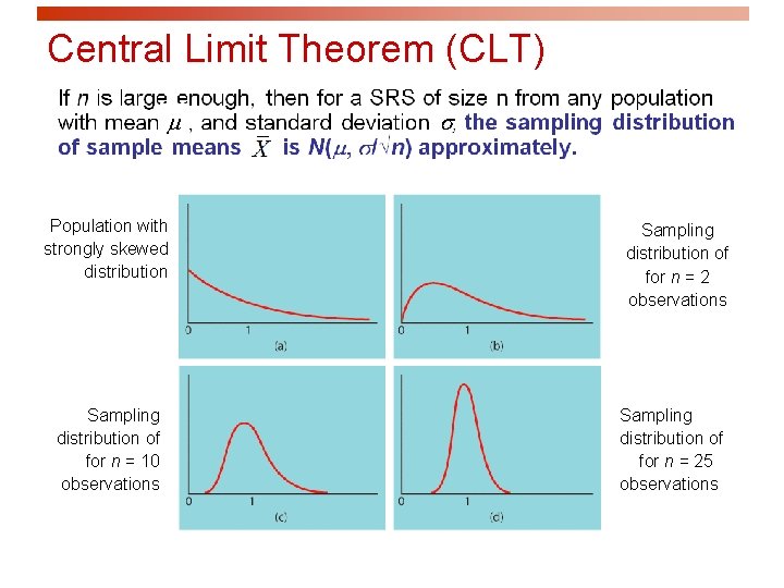
Central Limit Theorem (CLT) m Population with strongly skewed distribution Sampling distribution of for n = 10 observations s Sampling distribution of for n = 2 observations Sampling distribution of for n = 25 observations

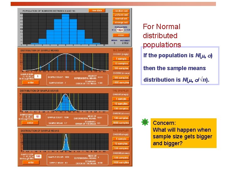
For Normal distributed populations If the population is N(m, s) then the sample means distribution is N(m, s/√n). Concern: What will happen when sample size gets bigger and bigger?

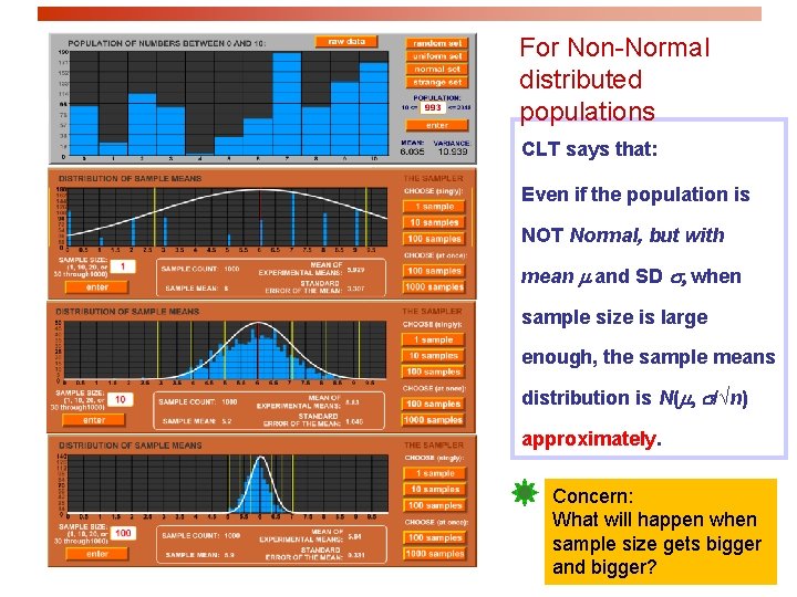
For Non-Normal distributed populations CLT says that: Even if the population is NOT Normal, but with mean m and SD s, when sample size is large enough, the sample means distribution is N(m, s/√n) approximately. Concern: What will happen when sample size gets bigger and bigger?

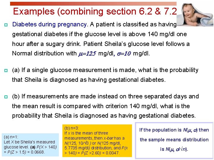
Examples (combining section 6. 2 & 7. 2) p Diabetes during pregnancy. A patient is classified as having gestational diabetes if the glucose level is above 140 mg/dl one hour after a sugary drink. Patient Sheila’s glucose level follows a Normal distribution with m=125 mg/dl, s=10 mg/dl. p (a) If a single glucose measurement is made, what is the probability that Sheila is diagnosed as having gestational diabetes. p (b) If measurements are made instead on three separated days and the mean result is compared with criterion 140 mg/dl, what is the probability that Sheila is diagnosed as having gestational diabetes. (a) n=1: Let X be Sheila’s measured glucose level. (a) P(X > 140) = P(Z > 1. 5) = 0. 0668. (b) n=3: If x is the mean of three measurements, then x-bar has a N(125, 10/√ 3 ) or N(125 mg/dl, 5. 7735 mg/dl) distribution, and P(x > 140) = P(Z >2. 60) = 0. 0047. If the population is N(m, s) then the sample means distribution is N(m, s/√n).

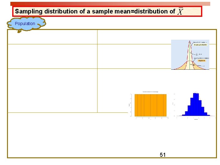
Sampling distribution of a sample mean=distribution of Population 51

How Sample Means Vary Around the Population Mean There are two main results about the sampling distribution of the sample mean: 1. One result provides formulas for its mean and standard deviation of the sampling distribution. 2. The other indicates that its shape is often approximately a normal distribution, as we observed in the previous section for the sample proportion. 52 Copyright © 2013, 2009, and 2007, Pearson Education, Inc.

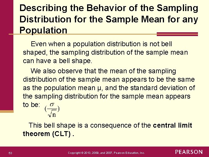
Describing the Behavior of the Sampling Distribution for the Sample Mean for any Population Even when a population distribution is not bell shaped, the sampling distribution of the sample mean can have a bell shape. We also observe that the mean of the sampling distribution of the sample mean appears to be the same as the population mean μ, and the standard deviation of the sampling distribution for the sample mean appears to be: This bell shape is a consequence of the central limit theorem (CLT). 53 Copyright © 2013, 2009, and 2007, Pearson Education, Inc.

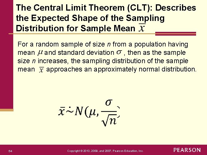
The Central Limit Theorem (CLT): Describes the Expected Shape of the Sampling Distribution for Sample Mean For a random sample of size n from a population having mean and standard deviation , then as the sample size n increases, the sampling distribution of the sample mean approaches an approximately normal distribution. 54 Copyright © 2013, 2009, and 2007, Pearson Education, Inc.

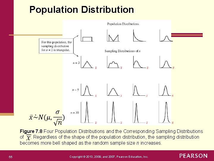
Population Distribution Figure 7. 8 Four Population Distributions and the Corresponding Sampling Distributions of. Regardless of the shape of the population distribution, the sampling distribution becomes more bell shaped as the random sample size n increases. 55 Copyright © 2013, 2009, and 2007, Pearson Education, Inc.

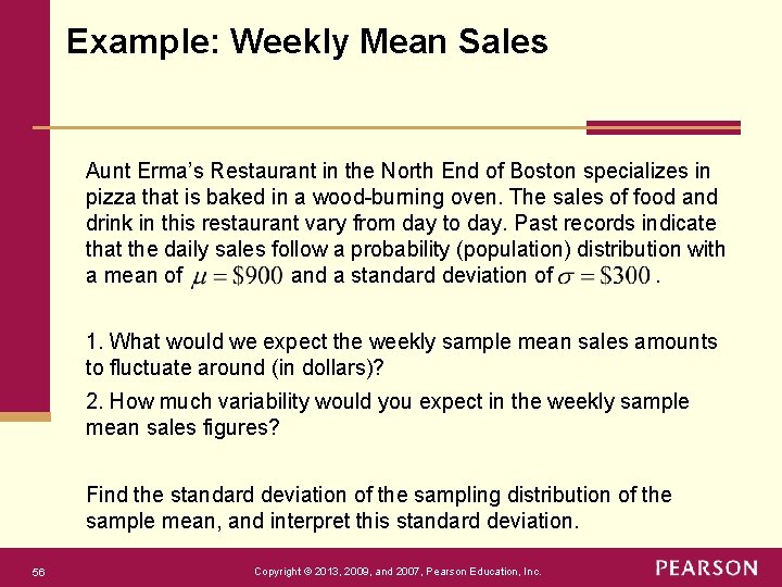
Example: Weekly Mean Sales Aunt Erma’s Restaurant in the North End of Boston specializes in pizza that is baked in a wood-burning oven. The sales of food and drink in this restaurant vary from day to day. Past records indicate that the daily sales follow a probability (population) distribution with a mean of and a standard deviation of. 1. What would we expect the weekly sample mean sales amounts to fluctuate around (in dollars)? 2. How much variability would you expect in the weekly sample mean sales figures? Find the standard deviation of the sampling distribution of the sample mean, and interpret this standard deviation. 56 Copyright © 2013, 2009, and 2007, Pearson Education, Inc.

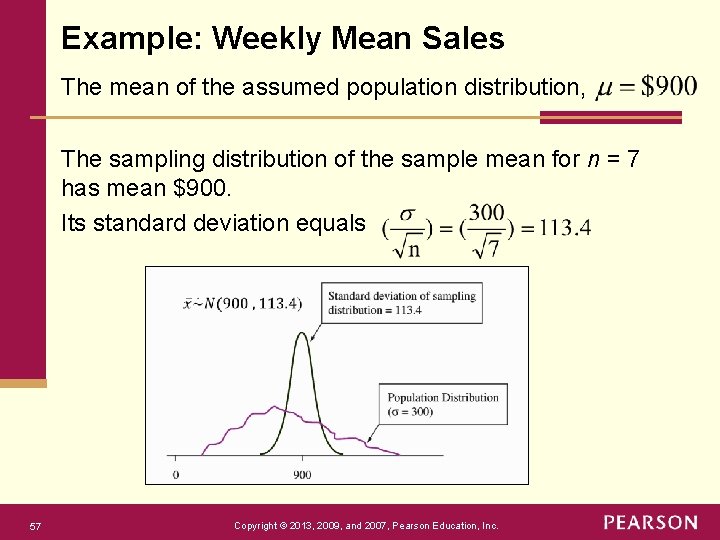
Example: Weekly Mean Sales The mean of the assumed population distribution, The sampling distribution of the sample mean for n = 7 has mean $900. Its standard deviation equals 57 Copyright © 2013, 2009, and 2007, Pearson Education, Inc.

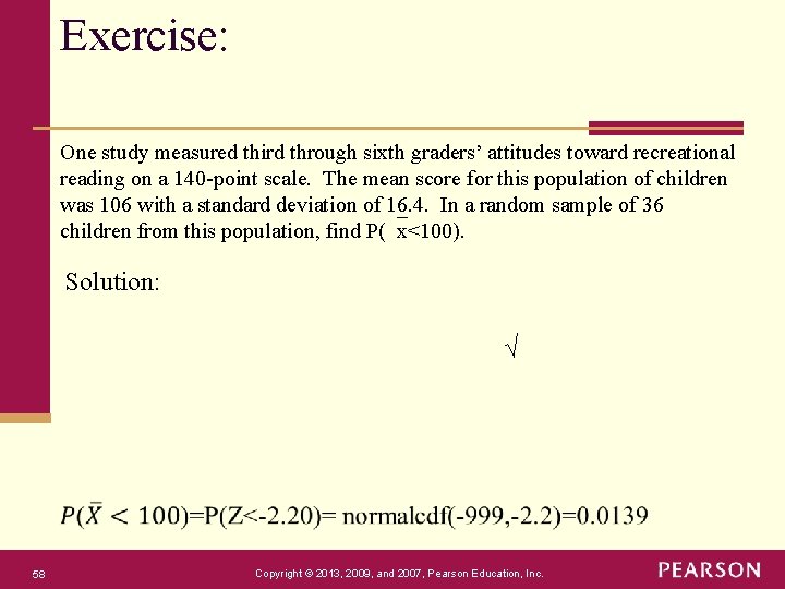
Exercise: One study measured third through sixth graders’ attitudes toward recreational reading on a 140 -point scale. The mean score for this population of children was 106 with a standard deviation of 16. 4. In a random sample of 36 children from this population, find P( x<100). Solution: √ 58 Copyright © 2013, 2009, and 2007, Pearson Education, Inc.

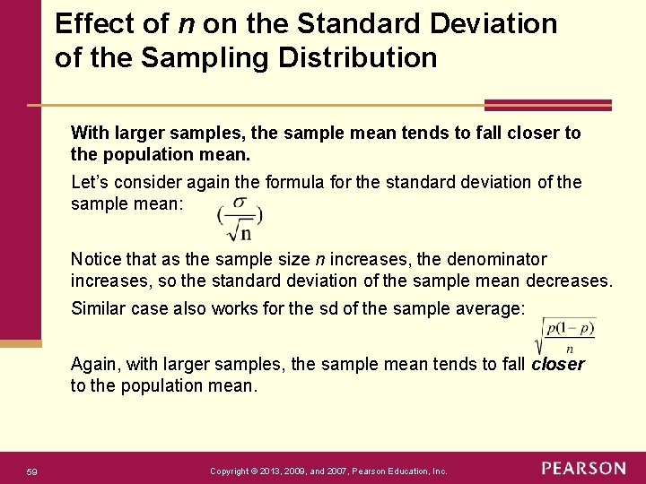
Effect of n on the Standard Deviation of the Sampling Distribution With larger samples, the sample mean tends to fall closer to the population mean. Let’s consider again the formula for the standard deviation of the sample mean: Notice that as the sample size n increases, the denominator increases, so the standard deviation of the sample mean decreases. Similar case also works for the sd of the sample average: Again, with larger samples, the sample mean tends to fall closer to the population mean. 59 Copyright © 2013, 2009, and 2007, Pearson Education, Inc.