Chapter 7 Risk Analysis Real Options and Capital

Chapter 7 Risk Analysis, Real Options and Capital Budgeting 7 -0

Key Concepts and Skills • Understand be able to apply scenario and sensitivity analysis • Understand the various forms of break-even analysis • Understand the importance of real options in capital budgeting • Understand decision trees 7 -1

Introduction • So far we've viewed cash flows as point estimates. Therefore, we could be making a wrong decision by using point estimates for NPV and IRR. • There is a chance that cash flow will take on a value significantly different from the expected value, this is Risk. • In the context of the capital budgeting projects discussed in this chapter, risk results almost entirely from the uncertainty about future cash flows, because the initial cash outflow is generally known. • This uncertainty (risk) results from a variety of factors including uncertainty about future revenues, expenditures and taxes. • The riskiness of a project's cash flows must be considered when deciding upon a project. 7 -2

Introduction • Therefore, to asses the risk of a potential project, the analyst needs to evaluate the riskiness of the cash inflows. • There are different approaches to evaluate the riskiness of the cash inflows including Sensitivity analysis, Scenario analysis, Break-Even analysis and decision trees. • Each allows us to look behind the NPV number to see how stable our estimates are. 7 -3

Sensitivity analysis and scenario analysis • One approach to evaluate the riskiness of the cash inflows is sensitivity analysis. • Sensitivity analysis: examines how sensitive a particular NPV calculation is to changes in underlying assumptions. • It is also known as what-if analysis and bob (best, optimistic and pessimistic) analysis. • Firm’s analysts prepare some optimistic and pessimistic forecasts for each of the different variables that determine the cash flows. 7 -4

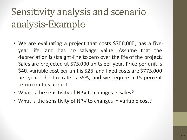
Sensitivity analysis and scenario analysis-Example • We are evaluating a project that costs $700, 000, has a fiveyear life, and has no salvage value. Assume that the depreciation is straight-line to zero over the life of the project. Sales are projected at $75, 000 units per year. Price per unit is $40, variable cost per unit is $25, and fixed costs are $775, 000 per year. The tax rate is 35%, and we require a 15 percent return on this project. • What is the sensitivity of NPV to changes in sales? • What is the sensitivity of NPV to changes in variable cost? 7 -5

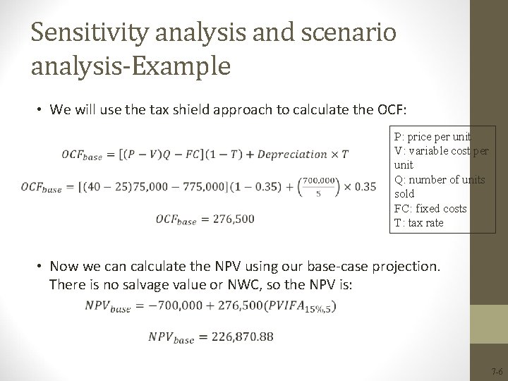
Sensitivity analysis and scenario analysis-Example • We will use the tax shield approach to calculate the OCF: P: price per unit V: variable cost per unit Q: number of units sold FC: fixed costs T: tax rate • Now we can calculate the NPV using our base-case projection. There is no salvage value or NWC, so the NPV is: 7 -6

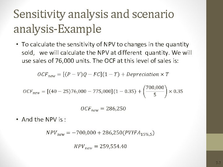
Sensitivity analysis and scenario analysis-Example • To calculate the sensitivity of NPV to changes in the quantity sold, we will calculate the NPV at different quantity. We will use sales of 76, 000 units. The OCF at this level of sales is: • And the NPV is : 7 -7

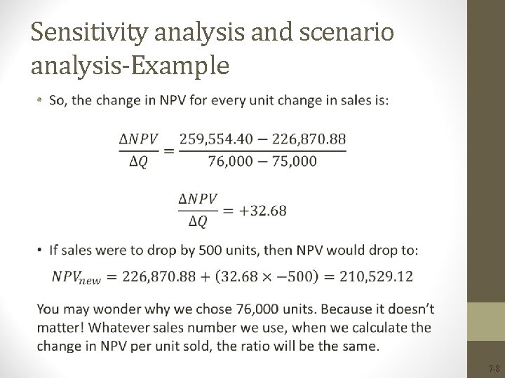
Sensitivity analysis and scenario analysis-Example • 7 -8

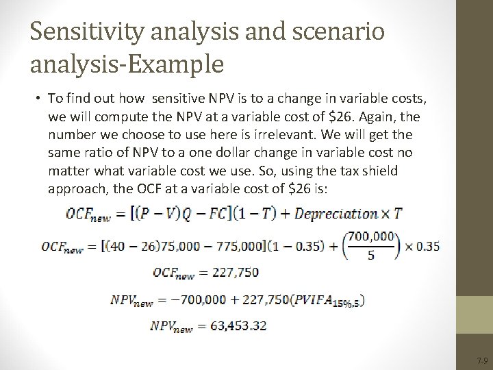
Sensitivity analysis and scenario analysis-Example • To find out how sensitive NPV is to a change in variable costs, we will compute the NPV at a variable cost of $26. Again, the number we choose to use here is irrelevant. We will get the same ratio of NPV to a one dollar change in variable cost no matter what variable cost we use. So, using the tax shield approach, the OCF at a variable cost of $26 is: 7 -9

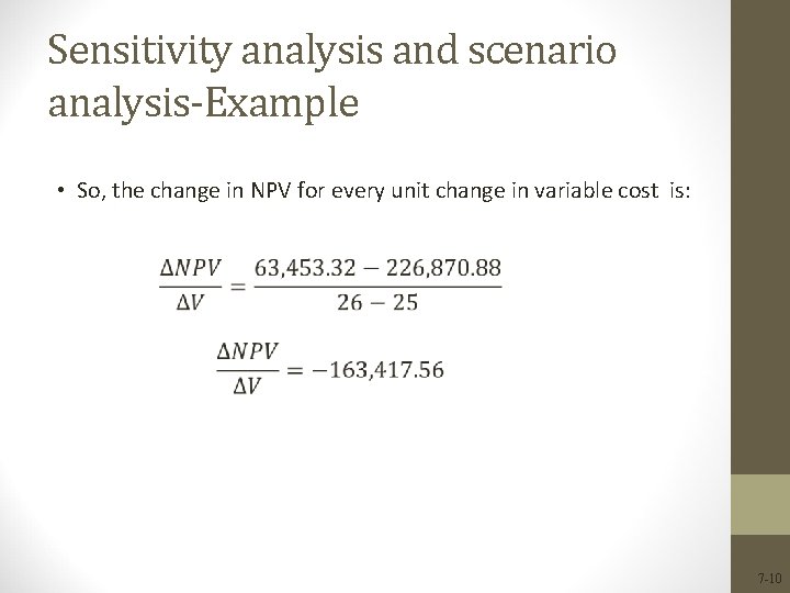
Sensitivity analysis and scenario analysis-Example • So, the change in NPV for every unit change in variable cost is: 7 -10

Sensitivity analysis and scenario analysis • Sensitivity analysis is widely used in practice as it: Ø indicates whether NPV should be trusted as it reduces the false sense associated with NPV. Ø shows where more information is needed. • However, sensitivity analysis suffers from some drawbacks. It treats each variable in isolation when in reality they are likely to be related. Ø It investigates the degree to which NPV depends on assumptions made about any singular critical variable. • Therefore, managers usually perform a variant approach which is scenario analysis. 7 -11

Sensitivity analysis and scenario analysis • Another approach to evaluate the riskiness of the cash inflows is scenario analysis. • It is a variation on sensitivity analysis. • It examines a number of different likely scenarios where each scenario involves a confluence of factors. • Involves selecting a worse, most likely and best case for each cash flow. • Recalculate the project's NPV (or IRR) under each scenario. 7 -12

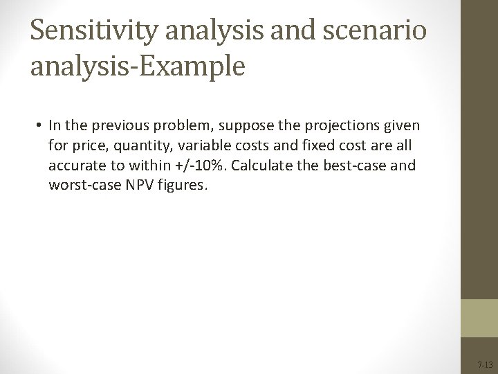
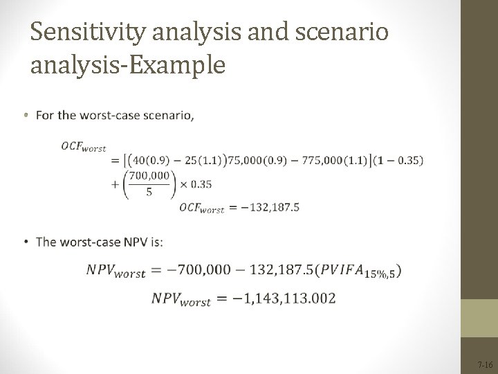
Sensitivity analysis and scenario analysis-Example • In the previous problem, suppose the projections given for price, quantity, variable costs and fixed cost are all accurate to within +/-10%. Calculate the best-case and worst-case NPV figures. 7 -13

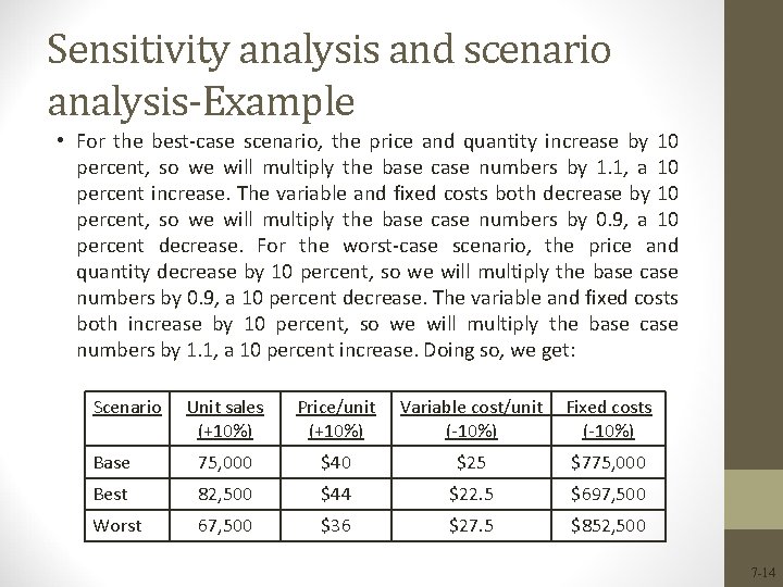
Sensitivity analysis and scenario analysis-Example • For the best-case scenario, the price and quantity increase by 10 percent, so we will multiply the base case numbers by 1. 1, a 10 percent increase. The variable and fixed costs both decrease by 10 percent, so we will multiply the base case numbers by 0. 9, a 10 percent decrease. For the worst-case scenario, the price and quantity decrease by 10 percent, so we will multiply the base case numbers by 0. 9, a 10 percent decrease. The variable and fixed costs both increase by 10 percent, so we will multiply the base case numbers by 1. 1, a 10 percent increase. Doing so, we get: Scenario Unit sales (+10%) Price/unit (+10%) Variable cost/unit Fixed costs (-10%) Base 75, 000 $40 $25 $775, 000 Best 82, 500 $44 $22. 5 $697, 500 Worst 67, 500 $36 $27. 5 $852, 500 7 -14

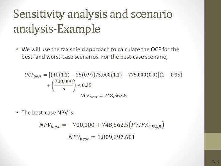
Sensitivity analysis and scenario analysis-Example • 7 -15

Sensitivity analysis and scenario analysis-Example • 7 -16

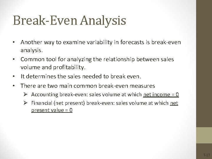
Break-Even Analysis • Another way to examine variability in forecasts is break-even analysis. • Common tool for analyzing the relationship between sales volume and profitability. • It determines the sales needed to break even. • There are two main common break-even measures Ø Accounting break-even: sales volume at which net income = 0 Ø Financial (net present) break-even: sales volume at which net present value = 0 7 -17

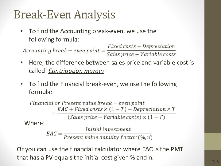
Break-Even Analysis • To find the Accounting break-even, we use the following formula: • Here, the difference between sales price and variable cost is called: Contribution margin • To find the Financial break-even, we use the following formula: Where: Or you can use the financial calculator where EAC is the PMT that has a PV equals the initial cost given % and n. 7 -18

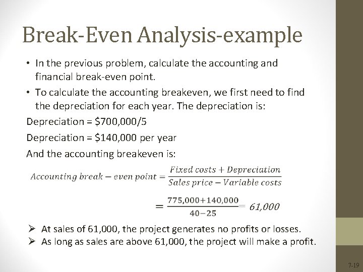
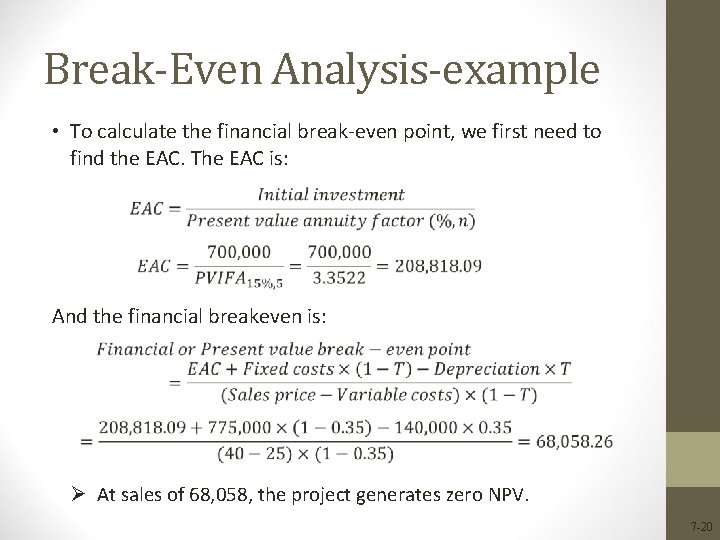
Break-Even Analysis-example • In the previous problem, calculate the accounting and financial break-even point. • To calculate the accounting breakeven, we first need to find the depreciation for each year. The depreciation is: Depreciation = $700, 000/5 Depreciation = $140, 000 per year And the accounting breakeven is: Ø At sales of 61, 000, the project generates no profits or losses. Ø As long as sales are above 61, 000, the project will make a profit. 7 -19

Break-Even Analysis-example • To calculate the financial break-even point, we first need to find the EAC. The EAC is: And the financial breakeven is: Ø At sales of 68, 058, the project generates zero NPV. 7 -20

Real Options • We have addressed the superiority of NPV over other approaches. However, many scholars have pointed out some concerns with traditional NPV. Traditional NPV ignores the adjustments that a firm can make after a project is accepted. These adjustments are called real options. • One of the fundamental insights of modern finance theory is that options have value. • The phrase “We are out of options” is surely a sign of trouble. • Because corporations make decisions in a dynamic environment, they have options that should be considered in project valuation. • Real option analysis is a methodology that allows us to value the strategic flexibility inherent in every project. 7 -21

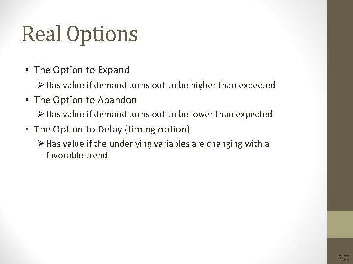
Real Options • The Option to Expand Ø Has value if demand turns out to be higher than expected • The Option to Abandon Ø Has value if demand turns out to be lower than expected • The Option to Delay (timing option) Ø Has value if the underlying variables are changing with a favorable trend 7 -22

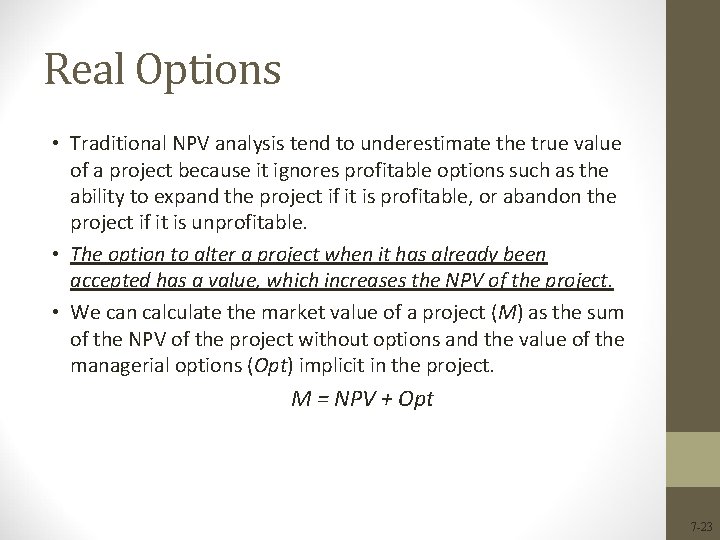
Real Options • Traditional NPV analysis tend to underestimate the true value of a project because it ignores profitable options such as the ability to expand the project if it is profitable, or abandon the project if it is unprofitable. • The option to alter a project when it has already been accepted has a value, which increases the NPV of the project. • We can calculate the market value of a project (M) as the sum of the NPV of the project without options and the value of the managerial options (Opt) implicit in the project. M = NPV + Opt 7 -23

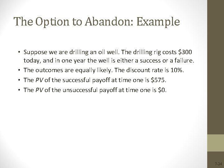
The Option to Abandon: Example • Suppose we are drilling an oil well. The drilling rig costs $300 today, and in one year the well is either a success or a failure. • The outcomes are equally likely. The discount rate is 10%. • The PV of the successful payoff at time one is $575. • The PV of the unsuccessful payoff at time one is $0. 7 -24

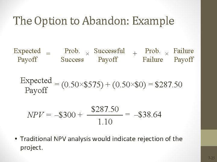
The Option to Abandon: Example Expected = Payoff Prob. × Successful + Prob. × Failure Success Payoff Failure Payoff Expected = (0. 50×$575) + (0. 50×$0) = $287. 50 Payoff NPV = –$300 + $287. 50 1. 10 = –$38. 64 • Traditional NPV analysis would indicate rejection of the project. 7 -25

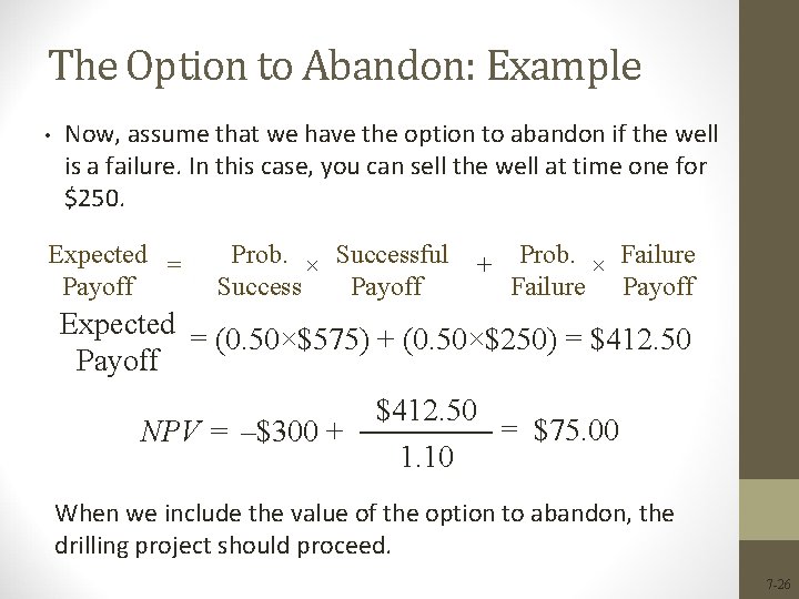
The Option to Abandon: Example • Now, assume that we have the option to abandon if the well is a failure. In this case, you can sell the well at time one for $250. Expected = Payoff Prob. × Successful + Prob. × Failure Success Payoff Failure Payoff Expected = (0. 50×$575) + (0. 50×$250) = $412. 50 Payoff NPV = –$300 + $412. 50 = $75. 00 1. 10 When we include the value of the option to abandon, the drilling project should proceed. 7 -26

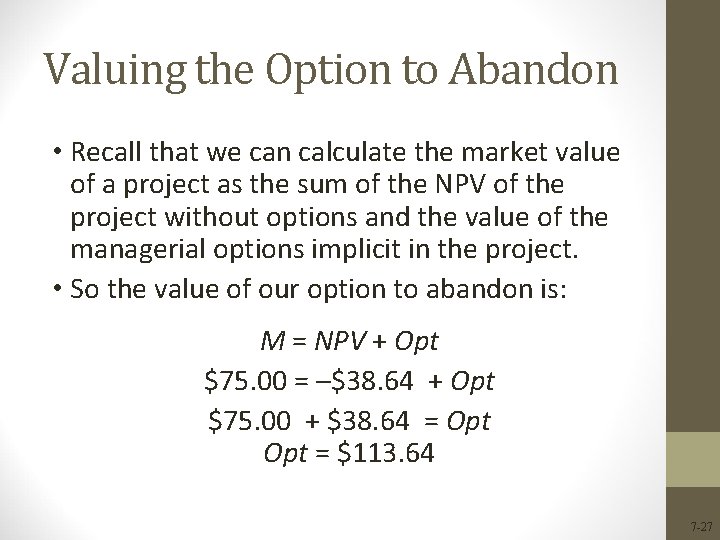
Valuing the Option to Abandon • Recall that we can calculate the market value of a project as the sum of the NPV of the project without options and the value of the managerial options implicit in the project. • So the value of our option to abandon is: M = NPV + Opt $75. 00 = –$38. 64 + Opt $75. 00 + $38. 64 = Opt = $113. 64 7 -27

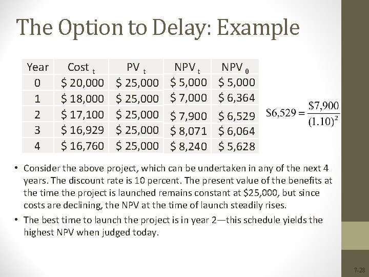
The Option to Delay: Example Year 0 1 2 3 4 Cost t $ 20, 000 $ 18, 000 $ 17, 100 $ 16, 929 $ 16, 760 PV t $ 25, 000 $ 25, 000 NPV t $ 5, 000 $ 7, 900 $ 8, 071 $ 8, 240 NPV 0 $ 5, 000 $ 6, 364 $ 6, 529 $ 6, 064 $ 5, 628 • Consider the above project, which can be undertaken in any of the next 4 years. The discount rate is 10 percent. The present value of the benefits at the time the project is launched remains constant at $25, 000, but since costs are declining, the NPV at the time of launch steadily rises. • The best time to launch the project is in year 2—this schedule yields the highest NPV when judged today. 7 -28

Decision Trees • Allow us to graphically represent the alternatives available to us in each period and the likely consequences of our actions • This graphical representation helps to identify the best course of action. 7 -29

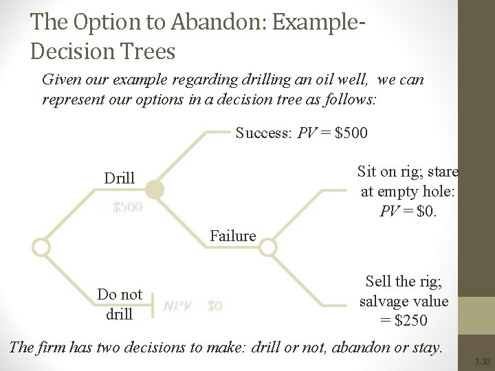
The Option to Abandon: Example. Decision Trees Given our example regarding drilling an oil well, we can represent our options in a decision tree as follows: Success: PV = $500 Sit on rig; stare at empty hole: PV = $0. Drill Failure Do not drill Sell the rig; salvage value = $250 The firm has two decisions to make: drill or not, abandon or stay. 7 -30

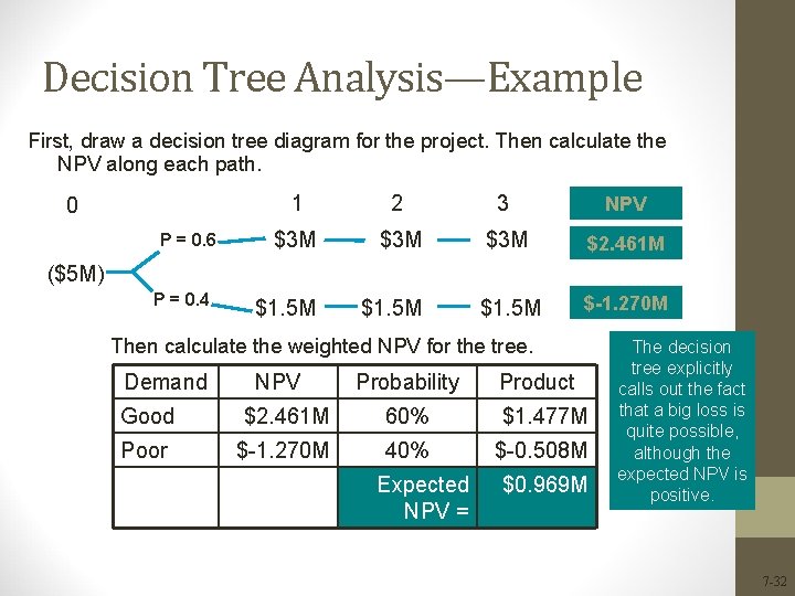
Decision Tree Analysis—Example The Wing Foot Shoe Company is considering a three-year project to market a running shoe based on new technology. Success depends on how well consumers accept the new idea and demand the product. Demand can vary from great to terrible, but for planning purposes management has collapsed that variation into just two possibilities, good and poor. A market study indicates a 60% probability that demand will be good and a 40% chance that it will be poor. It will cost $5 M to bring the new shoe to market. Cash flow estimates indicate inflows of $3 M per year for three years at full manufacturing capacity if demand is good, but just $1. 5 M per year if it’s poor. Wing Foot’s cost of capital is 10%. Analyze the project and develop a rough probability distribution for NPV. 7 -31

Decision Tree Analysis—Example First, draw a decision tree diagram for the project. Then calculate the NPV along each path. 0 P = 0. 6 1 2 3 NPV $3 M $3 M $2. 461 M $1. 5 M $-1. 270 M ($5 M) P = 0. 4 Then calculate the weighted NPV for the tree. Demand NPV Probability Product Good $2. 461 M 60% $1. 477 M Poor $-1. 270 M 40% $-0. 508 M Expected NPV = $0. 969 M The decision tree explicitly calls out the fact that a big loss is quite possible, although the expected NPV is positive. 7 -32