Chapter 7 Random Variables and Discrete probability Distributions
Chapter 7 Random Variables and Discrete probability Distributions 1
7. 2 Random Variables and Probability Distributions n n A random variable is a function or rule that assigns a numerical value to each simple event in a sample space. A random variable is related to a random experiment that is of interest for us. Ø n Since we don’t know the outcome of a random experiment, we don’t know what numerical value will be assigned to the random variable. There are two types of random variables: Ø Ø Discrete random variable. X=Outcome of tossing a dice X can be 1, 2, ---, 6. Continuous random variable. Weight of a person who are randomly selected from the population of Korean = any real number > 0. Weight =60. 1289 ------ Copyright © 2005 Brooks/Cole, a division of Thomson Learning, Inc. 2
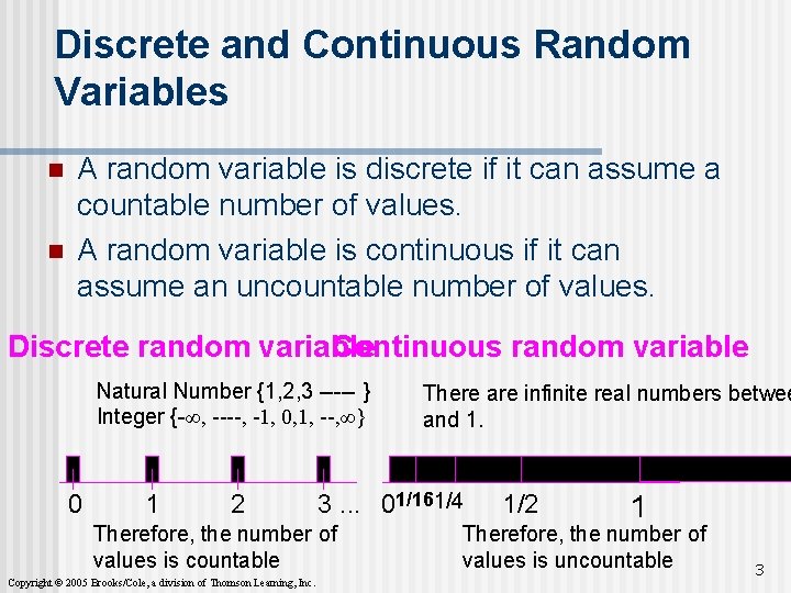
Discrete and Continuous Random Variables n n A random variable is discrete if it can assume a countable number of values. A random variable is continuous if it can assume an uncountable number of values. Discrete random variable Continuous random variable Natural Number {1, 2, 3 ----- } Integer {-∞, ----, -1, 0, 1, --, ∞} 0 1 2 3. . . 01/161/4 Therefore, the number of values is countable Copyright © 2005 Brooks/Cole, a division of Thomson Learning, Inc. There are infinite real numbers betwee and 1. 1/2 1 Therefore, the number of values is uncountable 3
Discrete Probability Distribution n A table, formula, or graph that lists all possible values a discrete random variable can assume, together with associated probabilities, is called a discrete probability distribution. n To calculate the probability that the random variable X assumes the value x, P(X = x), n n n add the probabilities of all the simple events for which X is equal to x, or Use probability calculation tools (tree diagram), Apply probability definitions Copyright © 2005 Brooks/Cole, a division of Thomson Learning, Inc. 4
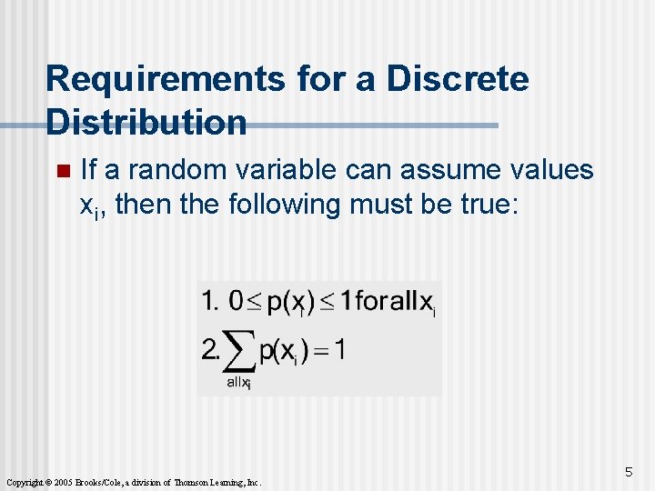
Requirements for a Discrete Distribution n If a random variable can assume values xi, then the following must be true: Copyright © 2005 Brooks/Cole, a division of Thomson Learning, Inc. 5
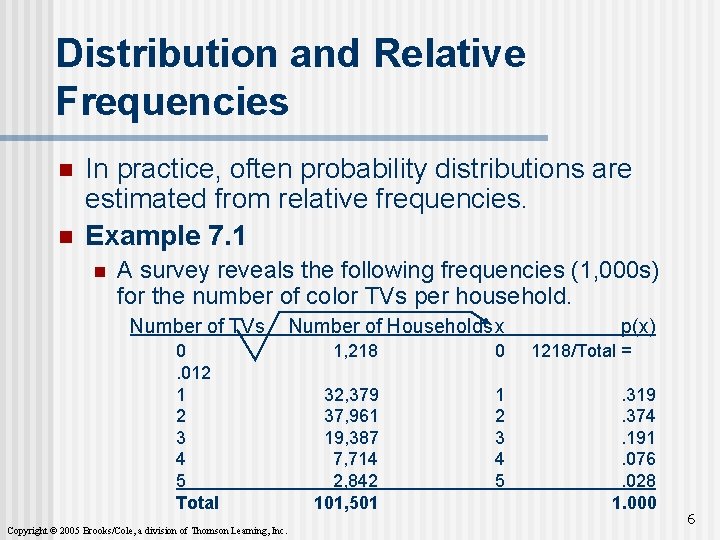
Distribution and Relative Frequencies n n In practice, often probability distributions are estimated from relative frequencies. Example 7. 1 n A survey reveals the following frequencies (1, 000 s) for the number of color TVs per household. Number of TVs 0. 012 1 2 3 4 5 Total Copyright © 2005 Brooks/Cole, a division of Thomson Learning, Inc. Number of Householdsx 1, 218 0 32, 379 37, 961 19, 387 7, 714 2, 842 101, 501 1 2 3 4 5 p(x) 1218/Total =. 319. 374. 191. 076. 028 1. 000 6
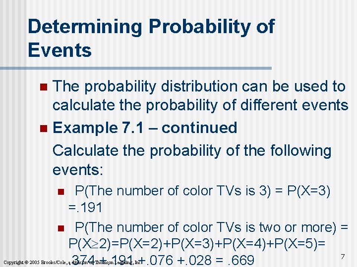
Determining Probability of Events The probability distribution can be used to calculate the probability of different events n Example 7. 1 – continued Calculate the probability of the following events: n P(The number of color TVs is 3) = P(X=3) =. 191 n P(The number of color TVs is two or more) = P(X³ 2)=P(X=2)+P(X=3)+P(X=4)+P(X=5)= 7. 374 +. 191 +. 076 +. 028 =. 669 n Copyright © 2005 Brooks/Cole, a division of Thomson Learning, Inc.
Developing a Probability Distribution Probability calculation techniques can be used to develop probability distributions. n Example 7. 2 n A mutual fund sales person knows that there is 20% chance of closing a sale on each call she makes. n What is the probability distribution of the number of sales if she plans to call three customers? n Copyright © 2005 Brooks/Cole, a division of Thomson Learning, Inc. 8
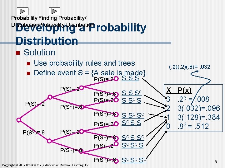
Probability Finding Probability/ Distribution. Probability Distribution Developing a Probability Distribution n Solution n n Use probability rules and trees Define event S = {A sale is made}. P(S)=. 2 P(SC)=. 8 P(S)=. 2 SSS P(SC)=. 8 P(S)=. 2 S S SC S P(SC)=. 8 P(S)=. 2 S S C SC SC S S P(SC)=. 8 P(S)=. 2 SC S S C SC SC S P(SC)=. 8 SC SC SC P(SC)=. 8 P(S)=. 2 P(SC)=. 8 Copyright © 2005 Brooks/Cole, a division of Thomson Learning, Inc. (. 2)(. 8)=. 032 X 3 2 1 0 P(x). 23 =. 008 3(. 032)=. 096 3(. 128)=. 384. 83 =. 512 9
7. 3 Describing the Population/ Probability Distribution The probability distribution represents a population. n We’re interested in describing the population by computing various parameters. n Specifically, we calculate the population mean and population variance. n Copyright © 2005 Brooks/Cole, a division of Thomson Learning, Inc. 10
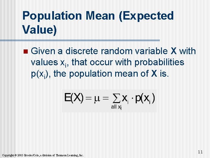
Population Mean (Expected Value) n Given a discrete random variable X with values xi, that occur with probabilities p(xi), the population mean of X is. Copyright © 2005 Brooks/Cole, a division of Thomson Learning, Inc. 11
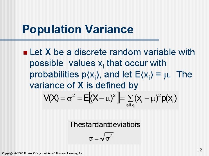
Population Variance n Let X be a discrete random variable with possible values xi that occur with probabilities p(xi), and let E(xi) = m. The variance of X is defined by Copyright © 2005 Brooks/Cole, a division of Thomson Learning, Inc. 12
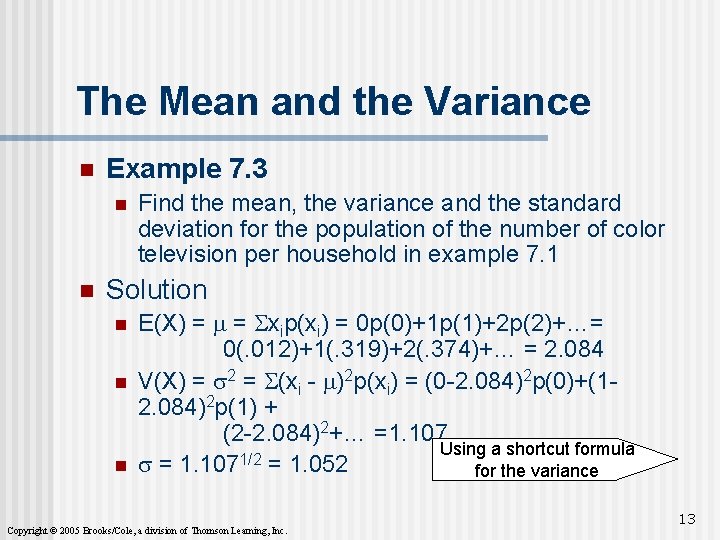
The Mean and the Variance n Example 7. 3 n n Find the mean, the variance and the standard deviation for the population of the number of color television per household in example 7. 1 Solution n E(X) = m = Sxip(xi) = 0 p(0)+1 p(1)+2 p(2)+…= 0(. 012)+1(. 319)+2(. 374)+… = 2. 084 V(X) = s 2 = S(xi - m)2 p(xi) = (0 -2. 084)2 p(0)+(12. 084)2 p(1) + (2 -2. 084)2+… =1. 107 Using a shortcut formula 1/2 s = 1. 107 = 1. 052 for the variance Copyright © 2005 Brooks/Cole, a division of Thomson Learning, Inc. 13
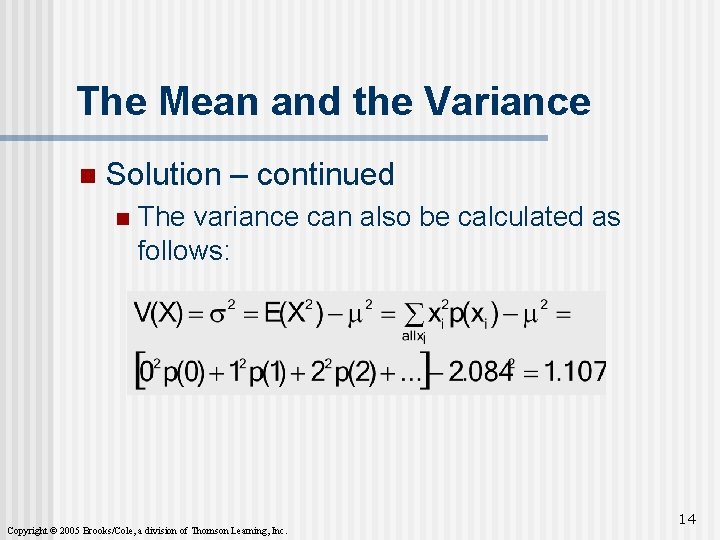
The Mean and the Variance n Solution – continued n The variance can also be calculated as follows: Copyright © 2005 Brooks/Cole, a division of Thomson Learning, Inc. 14
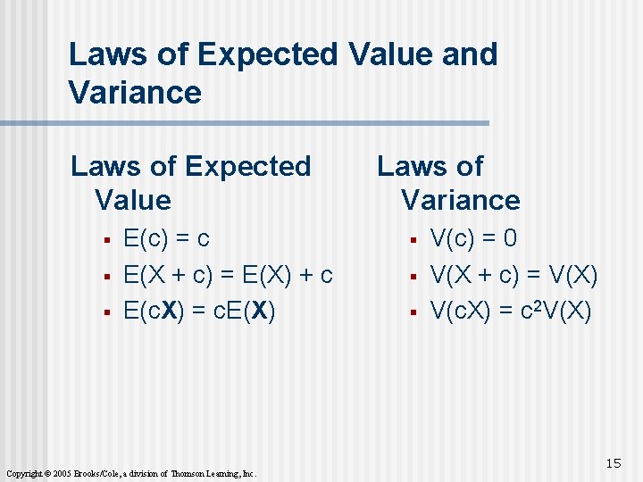
Laws of Expected Value and Variance Laws of Expected Value § § § E(c) = c E(X + c) = E(X) + c E(c. X) = c. E(X) Copyright © 2005 Brooks/Cole, a division of Thomson Learning, Inc. Laws of Variance § § § V(c) = 0 V(X + c) = V(X) V(c. X) = c 2 V(X) 15
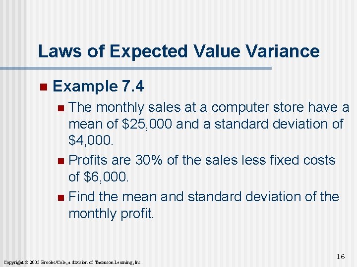
Laws of Expected Value Variance n Example 7. 4 The monthly sales at a computer store have a mean of $25, 000 and a standard deviation of $4, 000. n Profits are 30% of the sales less fixed costs of $6, 000. n Find the mean and standard deviation of the monthly profit. n Copyright © 2005 Brooks/Cole, a division of Thomson Learning, Inc. 16
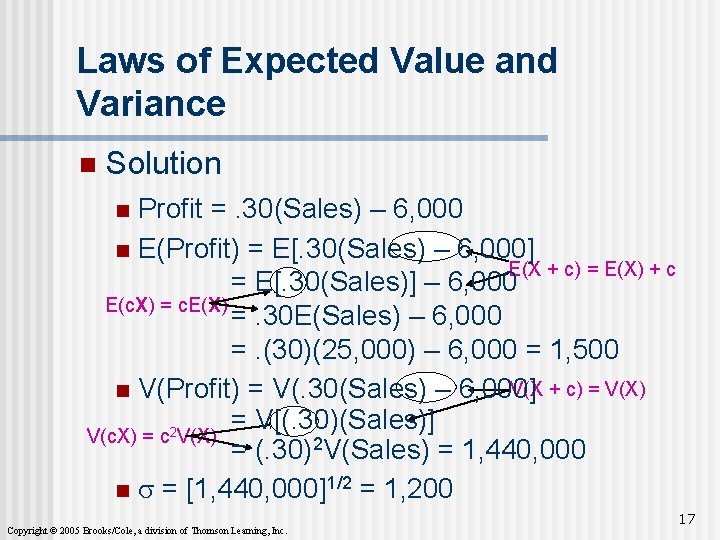
Laws of Expected Value and Variance n Solution Profit =. 30(Sales) – 6, 000 n E(Profit) = E[. 30(Sales) – 6, 000] E(X + c) = E(X) + c = E[. 30(Sales)] – 6, 000 E(c. X) = c. E(X) =. 30 E(Sales) – 6, 000 =. (30)(25, 000) – 6, 000 = 1, 500 V(X + c) = V(X) n V(Profit) = V(. 30(Sales) – 6, 000] = V[(. 30)(Sales)] V(c. X) = c 2 V(X) = (. 30)2 V(Sales) = 1, 440, 000 n s = [1, 440, 000]1/2 = 1, 200 n Copyright © 2005 Brooks/Cole, a division of Thomson Learning, Inc. 17
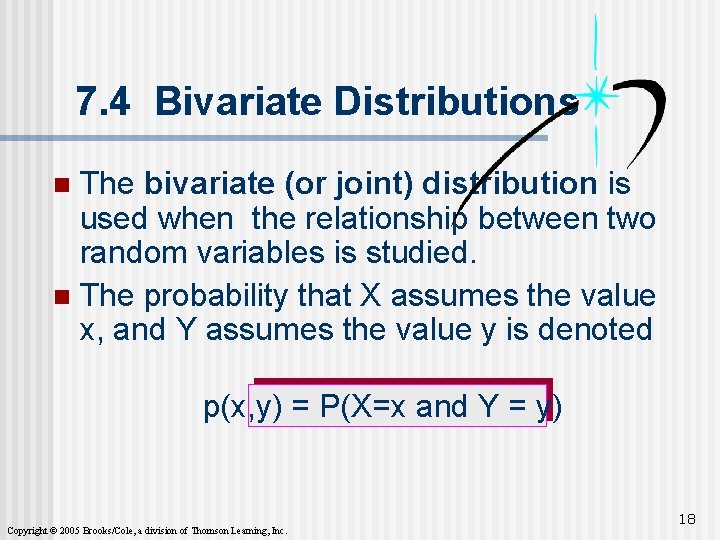
7. 4 Bivariate Distributions The bivariate (or joint) distribution is used when the relationship between two random variables is studied. n The probability that X assumes the value x, and Y assumes the value y is denoted n p(x, y) = P(X=x and Y = y) Copyright © 2005 Brooks/Cole, a division of Thomson Learning, Inc. 18
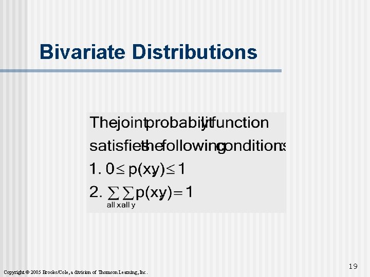
Bivariate Distributions Copyright © 2005 Brooks/Cole, a division of Thomson Learning, Inc. 19
Bivariate Distributions n Example 7. 5 n Xavier and Yvette are two real estate agents. Let X and Y denote the number of houses that Xavier and Yvette will sell next week, respectively. n The bivariate probability distribution is presented next. Copyright © 2005 Brooks/Cole, a division of Thomson Learning, Inc. 20
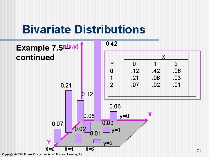
Bivariate Distributions 0. 42 7. 5 p(x, y) – Example continued X Y 0 1 2 0. 21 0. 12. 21. 07 1. 42. 06. 02 2. 06. 03. 01 0. 12 0. 06 0. 07 0. 02 0. 01 Y X=0 y=0 X 0. 03 y=1 y=2 X=1 Copyright © 2005 Brooks/Cole, a division of Thomson Learning, Inc. X=2 21
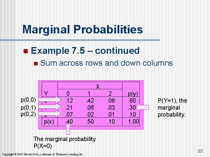
Marginal Probabilities n Example 7. 5 – continued n Sum across rows and down columns X p(0, 0) p(0, 1) p(0, 2) Y 0 1 2 p(x) 0. 12. 21. 07. 40 1. 42. 06. 02. 50 The marginal probability P(X=0) Copyright © 2005 Brooks/Cole, a division of Thomson Learning, Inc. 2. 06. 03. 01. 10 p(y). 60. 30. 10 1. 00 P(Y=1), the marginal probability. 22
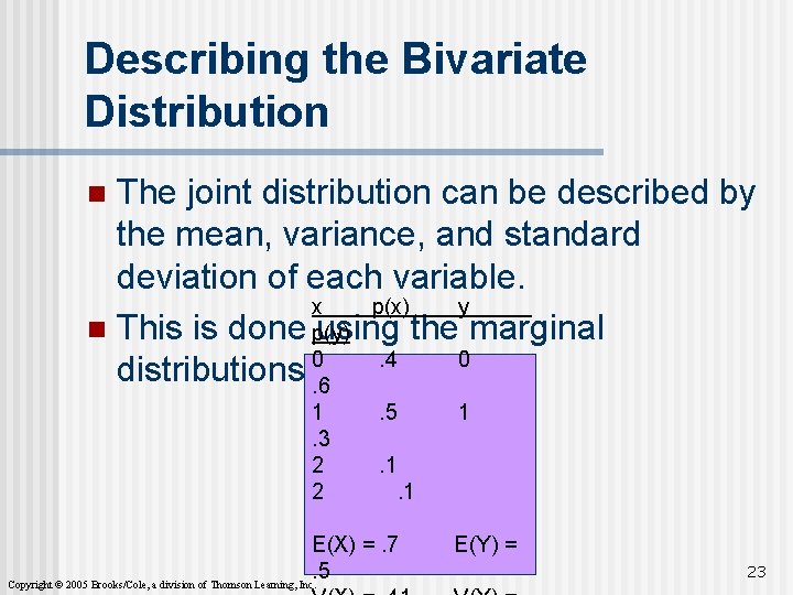
Describing the Bivariate Distribution The joint distribution can be described by the mean, variance, and standard deviation of each variable. x p(x) y n This is done p(y) using the marginal 0 distributions. 0. 6. 4 n 1. 3 2 2 . 5 1 . 1. 1 E(X) =. 7. 5 Copyright © 2005 Brooks/Cole, a division of Thomson Learning, Inc. E(Y) = 23
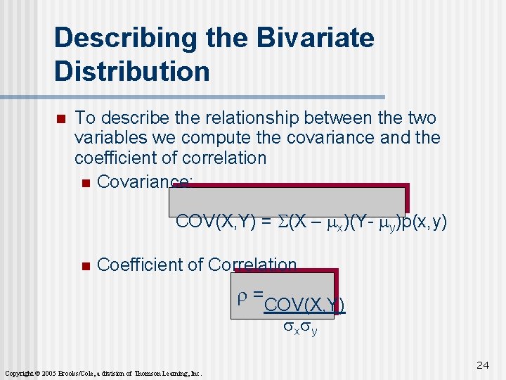
Describing the Bivariate Distribution n To describe the relationship between the two variables we compute the covariance and the coefficient of correlation n Covariance: COV(X, Y) = S(X – mx)(Y- my)p(x, y) n Coefficient of Correlation r =COV(X, Y) sxsy Copyright © 2005 Brooks/Cole, a division of Thomson Learning, Inc. 24
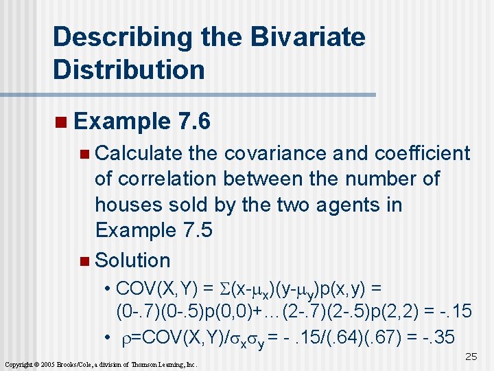
Describing the Bivariate Distribution n Example 7. 6 n Calculate the covariance and coefficient of correlation between the number of houses sold by the two agents in Example 7. 5 n Solution • COV(X, Y) = S(x-mx)(y-my)p(x, y) = (0 -. 7)(0 -. 5)p(0, 0)+…(2 -. 7)(2 -. 5)p(2, 2) = -. 15 • r=COV(X, Y)/sxsy = -. 15/(. 64)(. 67) = -. 35 Copyright © 2005 Brooks/Cole, a division of Thomson Learning, Inc. 25
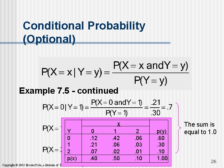
Conditional Probability (Optional) Example 7. 5 - continued X Y 0 1 2 p(x) Copyright © 2005 Brooks/Cole, a division of Thomson Learning, Inc. 0. 12. 21. 07. 40 1. 42. 06. 02. 50 2. 06. 03. 01. 10 p(y). 60. 30. 10 1. 00 The sum is equal to 1. 0 26
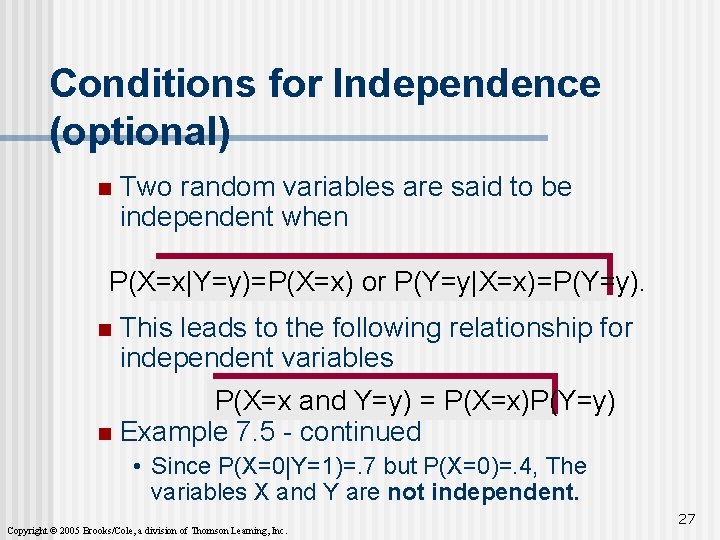
Conditions for Independence (optional) n Two random variables are said to be independent when P(X=x|Y=y)=P(X=x) or P(Y=y|X=x)=P(Y=y). n This leads to the following relationship for independent variables P(X=x and Y=y) = P(X=x)P(Y=y) n Example 7. 5 - continued • Since P(X=0|Y=1)=. 7 but P(X=0)=. 4, The variables X and Y are not independent. Copyright © 2005 Brooks/Cole, a division of Thomson Learning, Inc. 27
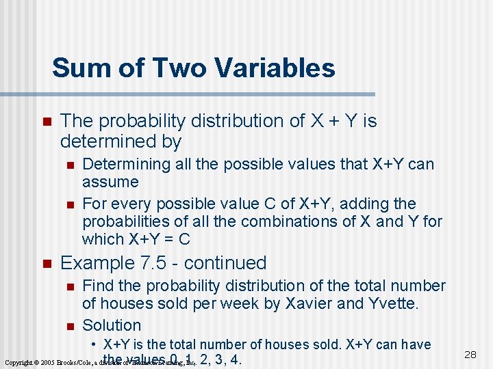
Sum of Two Variables n The probability distribution of X + Y is determined by n n n Determining all the possible values that X+Y can assume For every possible value C of X+Y, adding the probabilities of all the combinations of X and Y for which X+Y = C Example 7. 5 - continued n n Find the probability distribution of the total number of houses sold per week by Xavier and Yvette. Solution • X+Y is the total number of houses sold. X+Y can have the ofvalues 0, 1, Copyright © 2005 Brooks/Cole, a division Thomson Learning, Inc. 2, 3, 4. 28
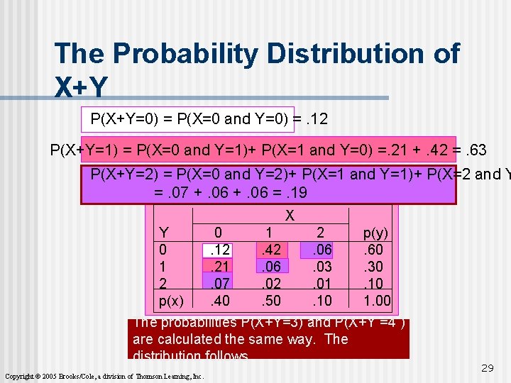
The Probability Distribution of X+Y P(X+Y=0) = P(X=0 and Y=0) =. 12 P(X+Y=1) = P(X=0 and Y=1)+ P(X=1 and Y=0) =. 21 +. 42 =. 63 P(X+Y=2) = P(X=0 and Y=2)+ P(X=1 and Y=1)+ P(X=2 and Y =. 07 +. 06 =. 19 X Y 0 1 2 p(y) 0. 12. 42. 06. 60 1. 21. 06. 03. 30 2. 07. 02. 01. 10 p(x). 40. 50. 10 1. 00 The probabilities P(X+Y=3) and P(X+Y =4 ) are calculated the same way. The distribution follows Copyright © 2005 Brooks/Cole, a division of Thomson Learning, Inc. 29
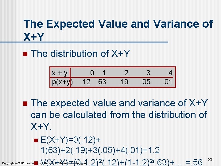
The Expected Value and Variance of X+Y n The distribution of X+Y x+y p(x+y) n 0 1. 12. 63 2. 19 3. 05 4. 01 The expected value and variance of X+Y can be calculated from the distribution of X+Y. E(X+Y)=0(. 12)+ 1(63)+2(. 19)+3(. 05)+4(. 01)=1. 2 n V(X+Y)=(0 -1. 2)2(. 12)+(1 -1. 2)2(. 63)+… =. 56 n Copyright © 2005 Brooks/Cole, a division of Thomson Learning, Inc. 30
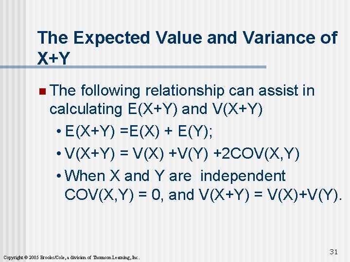
The Expected Value and Variance of X+Y n The following relationship can assist in calculating E(X+Y) and V(X+Y) • E(X+Y) =E(X) + E(Y); • V(X+Y) = V(X) +V(Y) +2 COV(X, Y) • When X and Y are independent COV(X, Y) = 0, and V(X+Y) = V(X)+V(Y). Copyright © 2005 Brooks/Cole, a division of Thomson Learning, Inc. 31
7. 6 The Binomial Distribution The binomial experiment can result in only one of two possible outcomes. n Typical cases where the binomial experiment applies: n A coin flipped results in heads or tails n An election candidate wins or loses n An employee is male or female n A car uses 87 octane gasoline, or another gasoline. n Copyright © 2005 Brooks/Cole, a division of Thomson Learning, Inc. 32
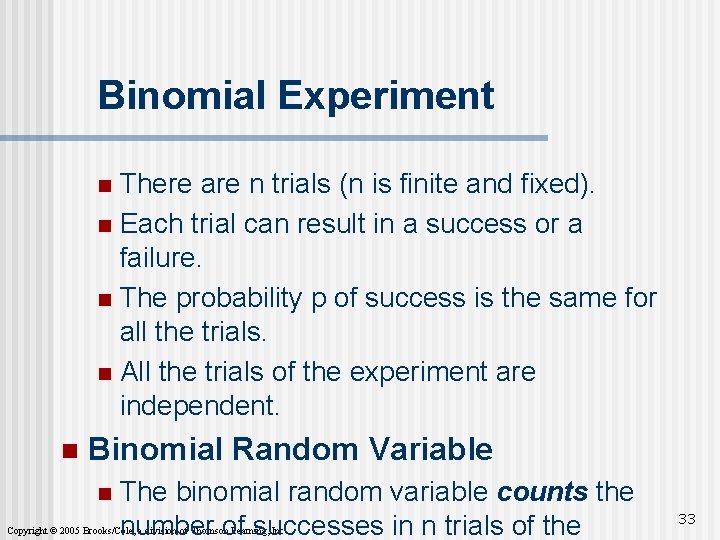
Binomial Experiment There are n trials (n is finite and fixed). n Each trial can result in a success or a failure. n The probability p of success is the same for all the trials. n All the trials of the experiment are independent. n n Binomial Random Variable n The binomial random variable counts the number of successes in n trials of the Copyright © 2005 Brooks/Cole, a division of Thomson Learning, Inc. 33
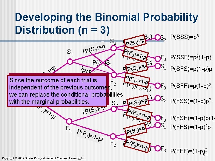
Developing the Binomial Probability Distribution (n = 3) ) S 1 p) = ) S | 1 S 2 (2 PP(S S 2 , S 1 S | 2 p P(S 3 )= S 3 P(SSS)=p 3 P(F | 1 -p 3 S 2 , S 1 )) S , F = | 2 p 1 ) S S ( ( 3 3 P P F 3 P(SSF)=p 2(1 -p) S 3 P(SFS)=p(1 -p)p P(S 3 P(F 3 )= P(S 2|S 1 PP(F p )1 = (F 2 |)S=1 ) 2 1 S ( p P(F ) P Since the outcome of each trial is F 2 P(F 3 =1 -p 3 |F 2 , S independent of the previous outcomes, 1) we can replace the conditional probabilities ) F , 1 S p | 2 = ) with the marginal probabilities. S(3 S 3 P( S 2 P(P F )=1)p 1 )= F | S 2 P ( 1 -p PP(S 2 P(F(F|3 )=1 -p 3 S 2 , F 1) ) F , 1 F | 2 F 1 (S(S 3 3)=p PP P(F |F-p 1 ) 2 )=21 F 2 PP(F(F 3|F ) -p 3 =21 , F 1 ) Copyright © 2005 Brooks/Cole, a division of Thomson Learning, Inc. F 3 P(SFF)=p(1 -p)2 S 3 P(FSS)=(1 -p)p 2 F 3 P(FSF)=(1 -p)p(1 S 3 P(FFS)=(1 -p)2 p F 3 P(FFF)=(1 -p)3 34
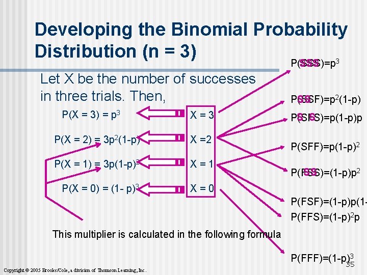
Developing the Binomial Probability Distribution (n = 3) 3 P(SSS)=p SSS Let X be the number of successes in three trials. Then, P(X = 3) = p 3 X=3 P(X = 2) = 3 p 2(1 -p) X =2 P(X = 1) = 3 p(1 -p)2 X=1 P(X = 0) = (1 - p)3 X=0 2(1 -p) P(SSF)=p SS S S P(SFS)=p(1 -p)p P(SFF)=p(1 -p)2 2 SS P(FSS)=(1 -p)p P(FSF)=(1 -p)p(1 P(FFS)=(1 -p)2 p This multiplier is calculated in the following formula P(FFF)=(1 -p)3 Copyright © 2005 Brooks/Cole, a division of Thomson Learning, Inc. 35
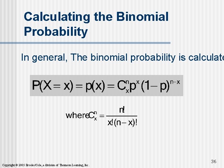
Calculating the Binomial Probability In general, The binomial probability is calculate Copyright © 2005 Brooks/Cole, a division of Thomson Learning, Inc. 36
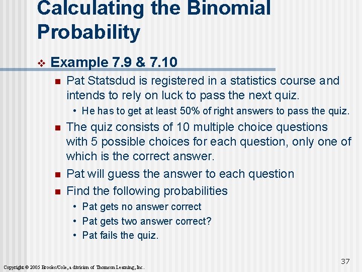
Calculating the Binomial Probability v Example 7. 9 & 7. 10 n Pat Statsdud is registered in a statistics course and intends to rely on luck to pass the next quiz. • He has to get at least 50% of right answers to pass the quiz. n n n The quiz consists of 10 multiple choice questions with 5 possible choices for each question, only one of which is the correct answer. Pat will guess the answer to each question Find the following probabilities • Pat gets no answer correct • Pat gets two answer correct? • Pat fails the quiz. Copyright © 2005 Brooks/Cole, a division of Thomson Learning, Inc. 37
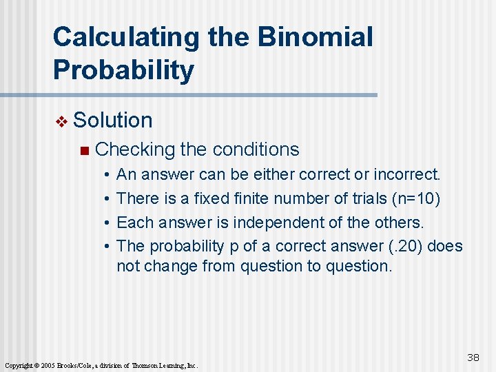
Calculating the Binomial Probability v Solution n Checking the conditions • • An answer can be either correct or incorrect. There is a fixed finite number of trials (n=10) Each answer is independent of the others. The probability p of a correct answer (. 20) does not change from question to question. Copyright © 2005 Brooks/Cole, a division of Thomson Learning, Inc. 38
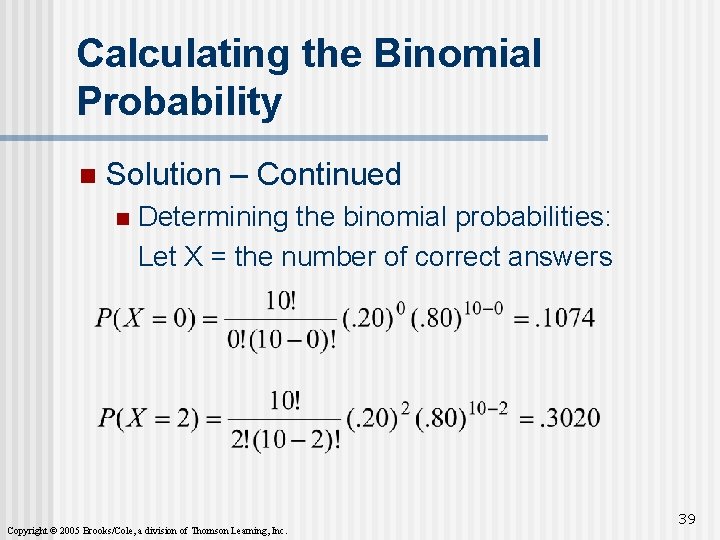
Calculating the Binomial Probability n Solution – Continued n Determining the binomial probabilities: Let X = the number of correct answers Copyright © 2005 Brooks/Cole, a division of Thomson Learning, Inc. 39
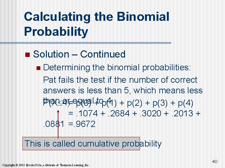
Calculating the Binomial Probability n Solution – Continued n Determining the binomial probabilities: Pat fails the test if the number of correct answers is less than 5, which means less than or=equal 4. + p(2) + p(3) + p(4) P(X£ 4) p(0) +top(1) =. 1074 +. 2684 +. 3020 +. 2013 +. 0881 =. 9672 This is called cumulative probability Copyright © 2005 Brooks/Cole, a division of Thomson Learning, Inc. 40
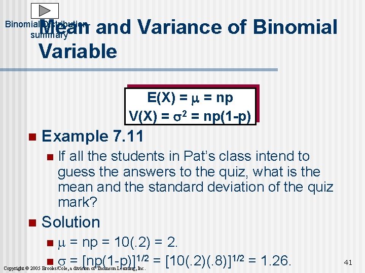
Mean and Variance of Binomial Variable Binomial Distributionsummary E(X) = m = np V(X) = s 2 = np(1 -p) n Example 7. 11 n n If all the students in Pat’s class intend to guess the answers to the quiz, what is the mean and the standard deviation of the quiz mark? Solution m = np = 10(. 2) = 2. n s = [np(1 -p)]1/2 = [10(. 2)(. 8)]1/2 = 1. 26. n Copyright © 2005 Brooks/Cole, a division of Thomson Learning, Inc. 41
- Slides: 41