Chapter 7 Numerical Differentiation and Integration INTRODUCTION DIFFERENTIATION

Chapter 7 Numerical Differentiation and Integration

INTRODUCTION DIFFERENTIATION USING DIFFERENCE OPREATORS DIFFERENTIATION USING INTERPOLATION RICHARDSON’S EXTRAPOLATION METHOD NUMERICAL INTEGRATION

NEWTON-COTES INTEGRATION FORMULAE THE TRAPEZOIDAL RULE ( COMPOSITE FORM ) SIMPSON’S RULES ( COMPOSITE FORM ) ROMBERG’S INTEGRATION DOUBLE INTEGRATION

Basic Issues in Integration What does an integral represent? = AREA = VOLUME

Basic definition of an integral: : = = sum of Height x Width

Objective: Evaluate I = without doing calculation analytically. When would we want to do this?

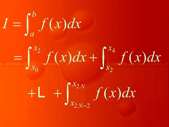
NUMERICAL INTEGRATION Consider the definite integral

where f (x) is known either explicitly or is given as a table of values corresponding to some values of x, whether equispaced or not. Integration of such functions can be carried out using numerical techniques.

Y y = f(x) (x 1, y 1) (x 2, y 2) (x 0, y 0) y 0 y 1 y 2 y 3 yn-1 yn O X x 0 = a x 1 x 2 x 3 xn-1 xn = b

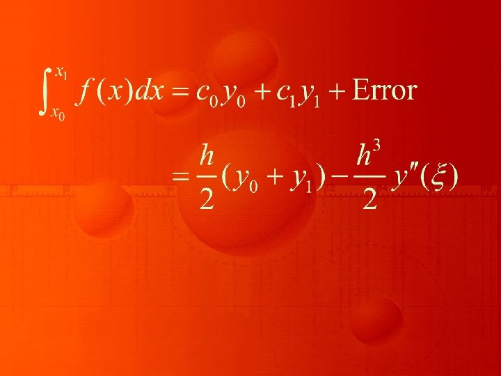
This area is approximated by the trapezium formed by replacing the curve with its secant line drawn between the end points (x 0, y 0) and (x 1, y 1).

Then, if n = 2, the integration takes the form

This is known as Simpson’s 1/3 rule. Geometrically, this equation represents the area between the curve y = f (x), the x-axis and the ordinates at x = x 0 and x 2 after replacing the arc of the curve between (x 0, y 0) and (x 2, y 2) by an arc of a quadratic polynomial as in the figure

Y y = f(x) (x 2, y 2) (x 0, y 0) y 0 y 1 y 2 O X x 0 = a x 1 x 2 x 3 xn-1 xn = b

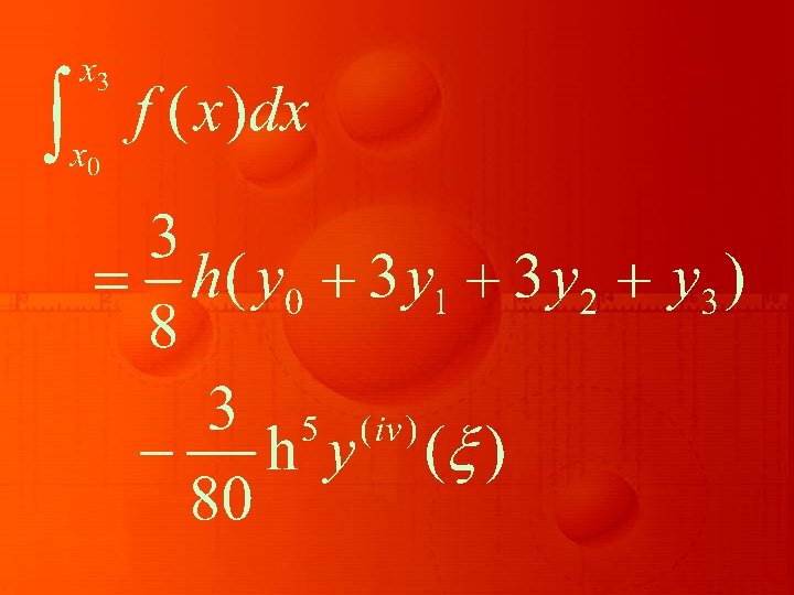
Thus Simpson’s 1/3 rule is based on fitting three points with a quadratic. Similarly, for n = 3, the integration is found to be

This is known as Simpson’s 3/8 rule, which is based on fitting four points by a cubic. Still higher order Newton. Cotes integration formulae can be derived for large values of n.

But for all practical purposes, Simpson’s 1/3 rule is found to be sufficiently accurate.

The Trapezoidal Rule (Composite Form) The Newton-Cotes formula is based on approximating y = f (x) between (x 0, y 0) and (x 1, y 1)

by a straight line, thus forming a trapezium, is called trapezoidal rule. In order to evaluate the definite integral

we divide the interval [a, b] into n sub-intervals, each of size h = (b – a)/n and denote the sub-intervals by [x 0, x 1], [x 1, x 2], …, [xn-1, xn], such that x 0 = a and xn = b and xk = x 0 + kh, k = 1, 2, …, n – 1.

Thus, we can write the above definite integral as a sum. Therefore,

The area under the curve in each sub-interval is approximated by a trapezium. The integral I, which represents an area between the curve y = f (x), the x-axis and the ordinates at x = x 0

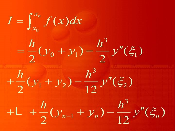
and x = xn is obtained by adding all the trapezoidal areas in each sub-interval. Now, using the trapezoidal rule into equation:

we get

where xk-1< ξ < xk, for k = 1, 2, …, n – 1. Thus, we arrive at the result

where the error term En is given by

Equation represents trapezoidal rule over [x 0, which is also called composite form of trapezoidal rule. the xn], the

The error term given by Equation:

is called the global error. However, if we assume that is continuous over [x 0, xn] then there exists some ξ in [x 0, xn] such that xn = x 0 + nh and

Then the global error can be conveniently written as O(h 2).

Simpson’s Rules (Composite Forms) In deriving equation. ,

the Simpson’s 1/3 rule, we have used two sub-intervals of equal width. In order to get a composite formula, we shall divide the interval of integration [a, b] Into an even number of subintervals say 2 N,

each of width (b – a)/2 N, thereby we have x 0 = a, x 1, …, x 2 N = b and xk =x 0 +kh, k = 1, 2, … (2 N – 1). Thus, the definite integral I can be written as

Applying Simpson’s 1/3 rule as in equation

to each of the integrals on the right-hand side of the above equation, we obtain

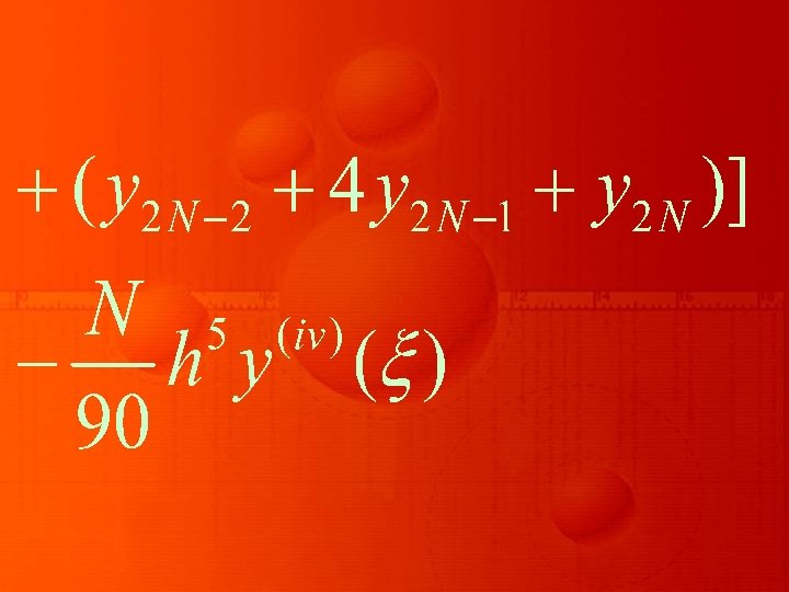
That is,

This formula is called composite Simpson’s 1/3 rule. The error term E, which is also called global error, is given by

for some ξ in [x 0, x 2 N]. Thus, in Simpson’s 1/3 rule, the global error is of O(h 2). Similarly in deriving composite Simpson’s 3/8 rule, we divide the interval of integration into n subintervals, where n is divisible by 3,

and applying the integration formula

to each of the integral given below

we obtain the composite form of Simpson’s 3/8 rule as

with the global error E given by

It may be noted that the global error in Simpson’s 1/3 and 3/8 rules are of the same order. However, if we consider the magnitudes of the error terms, we notice that Simpson’s 1/3 rule is superior to Simpson’s 3/8 rule. For illustration, we consider few examples.

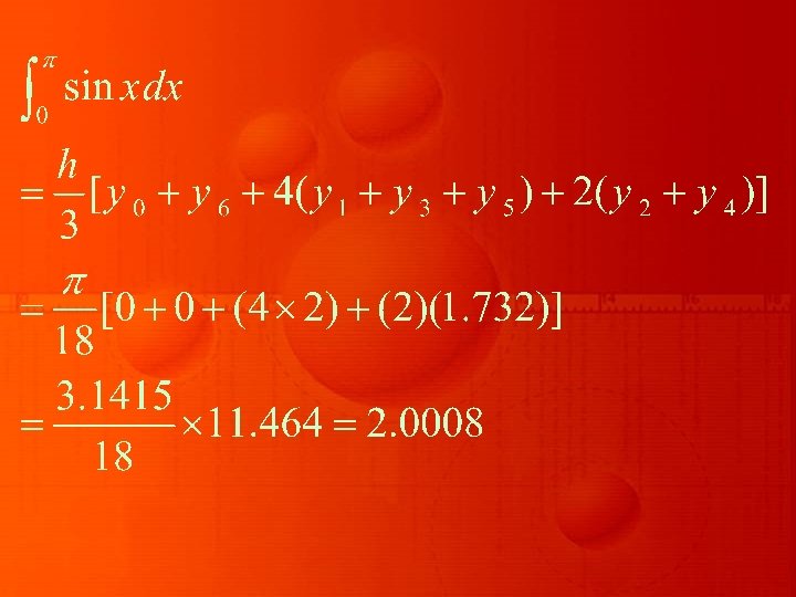
Example Find the approximate value of using (i) trapezoidal rule

(ii) Simpson’s 1/3 rule by dividing the range of integration into six equal parts. Calculate the percentage error from its true value in both the cases.

Solution We shall first atdivide the range of integration into six equal parts so that each part is of width and write down the table of values:

x 0 π/6 π/3 π/2 2π/3 5π/6 π y = sin x 0. 0 0. 5 0. 8660 1. 0 0. 8660 0. 5 0.

Applying trapezoidal rule, we have

Here, h, the width of the interval is π /6. Therefore,

Applying Simpson’s 1/3 rule We have

But the actual value of the integral is Hence, in the case of trapezoidal rule

The percentage of error While in the case of Simpson’s rule the percentage error is (sign ignored)