Chapter 7 Generating and Processing Random Signals B

Chapter 7 Generating and Processing Random Signals 第一組 電機四 B 93902016 蔡馭理 資 四 B 93902076 林宜鴻 1

Outline l Stationary and Ergodic Process l Uniform Random Number Generator l Mapping Uniform RVs to an Arbitrary pdf l Generating Uncorrelated Gaussian RV l Generating correlated Gaussian RV l PN Sequence Generators l Signal processing 2

Random Number Generator l Noise, interference l Random Number Generatorcomputational or physical device designed to generate a sequence of numbers or symbols that lack any pattern, i. e. appear random, pseudo-random sequence l MATLAB - rand(m, n) , randn(m, n) 3

Stationary and Ergodic Process strict-sense stationary (SSS) l wide-sense stationary (WSS) l Gaussian SSS =>WSS ; WSS=>SSS l Time average v. s ensemble average l The ergodicity requirement is that the ensemble average coincide with the time average l Sample function generated to represent signals, noise, interference should be ergodic l 4

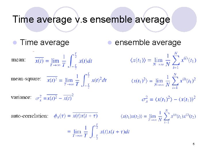
Time average v. s ensemble average l Time average l ensemble average 5

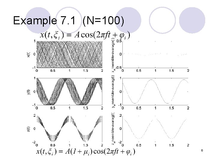
Example 7. 1 (N=100) 6

Uniform Random Number Genrator l Generate a random variable that is uniformly distributed on the interval (0, 1) l Generate a sequence of numbers (integer) between 0 and M and the divide each element of the sequence by M l The most common technique is linear congruence genrator (LCG) 7

Linear Congruence l LCG is defined by the operation: xi+1=[axi+c]mod(m) l x 0 is seed number of the generator l a, c, m, x 0 are integer l Desirable property- full period 8

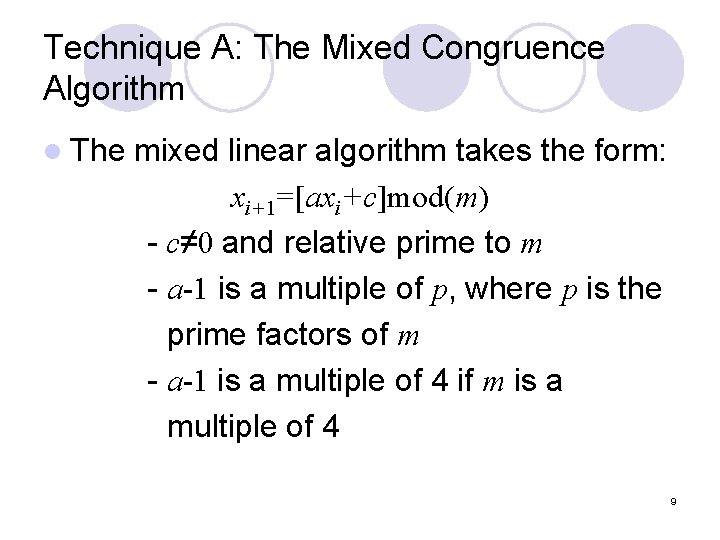
Technique A: The Mixed Congruence Algorithm l The mixed linear algorithm takes the form: xi+1=[axi+c]mod(m) - c≠ 0 and relative prime to m - a-1 is a multiple of p, where p is the prime factors of m - a-1 is a multiple of 4 if m is a multiple of 4 9

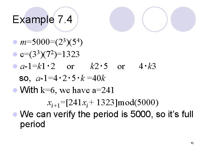
Example 7. 4 l m=5000=(23)(54) l c=(33)(72)=1323 l a-1=k 1‧ 2 or k 2‧ 5 or 4‧k 3 so, a-1=4‧ 2‧ 5‧k =40 k l With k=6, we have a=241 xi+1=[241 xi+ 1323]mod(5000) l We can verify the period is 5000, so it’s full period 10

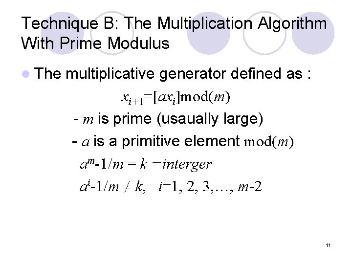
Technique B: The Multiplication Algorithm With Prime Modulus l The multiplicative generator defined as : xi+1=[axi]mod(m) - m is prime (usaually large) - a is a primitive element mod(m) am-1/m = k =interger ai-1/m ≠ k, i=1, 2, 3, …, m-2 11

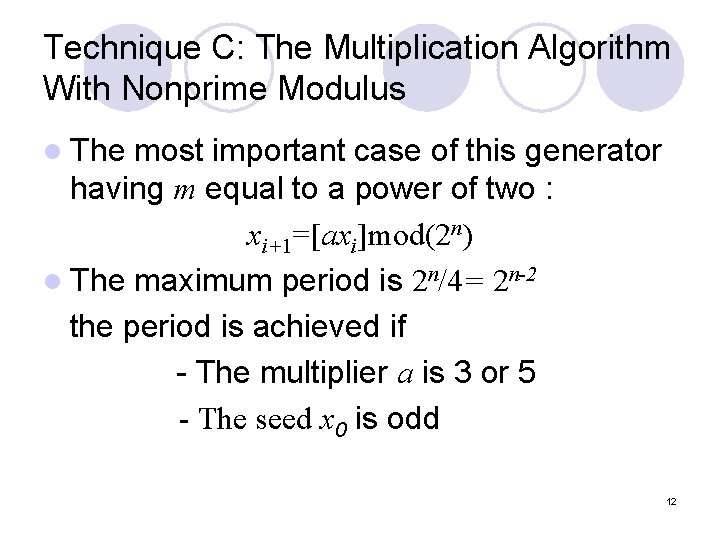
Technique C: The Multiplication Algorithm With Nonprime Modulus l The most important case of this generator having m equal to a power of two : xi+1=[axi]mod(2 n) l The maximum period is 2 n/4= 2 n-2 the period is achieved if - The multiplier a is 3 or 5 - The seed x 0 is odd 12

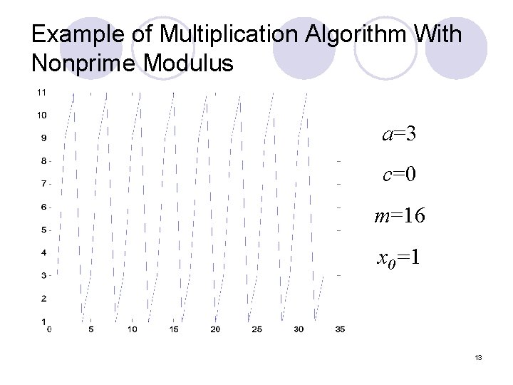
Example of Multiplication Algorithm With Nonprime Modulus a=3 c=0 m=16 x 0=1 13

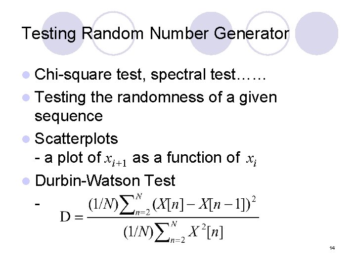
Testing Random Number Generator l Chi-square test, spectral test…… l Testing the randomness of a given sequence l Scatterplots - a plot of xi+1 as a function of xi l Durbin-Watson Test 14

Scatterplots Example 7. 5 (i) rand(1, 2048) (ii)xi+1=[65 xi+1] mod(2048) (iii)xi+1=[1229 xi+ 1]mod(2048) 15

Durbin-Watson Test (1) Let X = X[n] & Y = X[n-1] Assume X[n] and X[n-1] are correlated and X[n] is an ergodic process Let 16

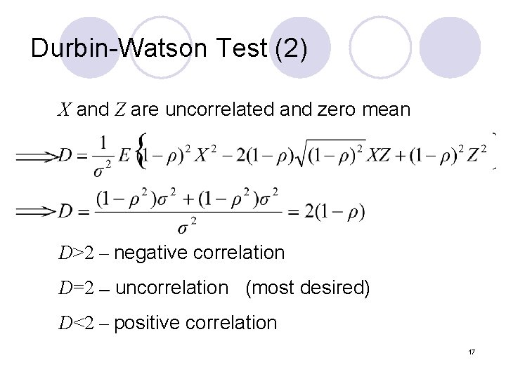
Durbin-Watson Test (2) X and Z are uncorrelated and zero mean D>2 – negative correlation D=2 –- uncorrelation (most desired) D<2 – positive correlation 17

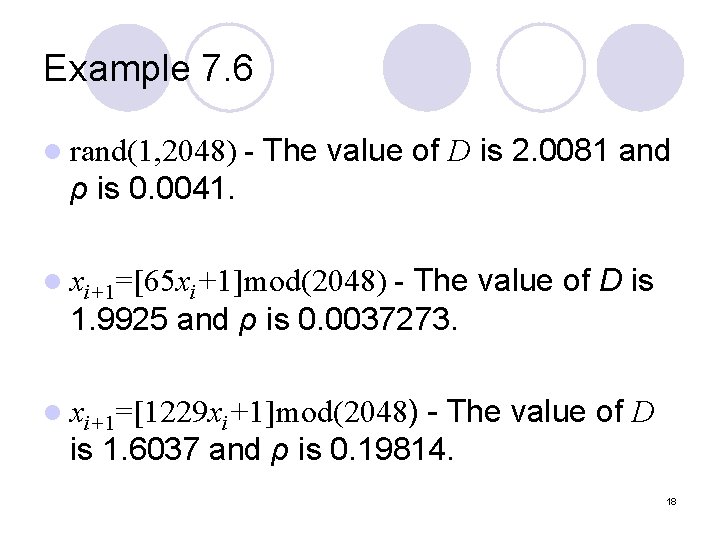
Example 7. 6 l rand(1, 2048) - The value of D is 2. 0081 and ρ is 0. 0041. - The value of D is 1. 9925 and ρ is 0. 0037273. l xi+1=[65 xi+1]mod(2048) - The value of D is 1. 6037 and ρ is 0. 19814. l xi+1=[1229 xi+1]mod(2048) 18

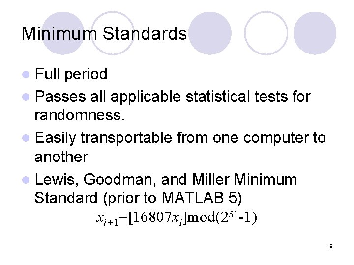
Minimum Standards l Full period l Passes all applicable statistical tests for randomness. l Easily transportable from one computer to another l Lewis, Goodman, and Miller Minimum Standard (prior to MATLAB 5) xi+1=[16807 xi]mod(231 -1) 19

Mapping Uniform RVs to an Arbitrary pdf l The cumulative distribution for the target random variable is known in closed form – Inverse Transform Method l The pdf of target random variable is known in closed form but the CDF is not known in closed form – Rejection Method l Neither the pdf nor CDF are known in closed form – Histogram Method 20

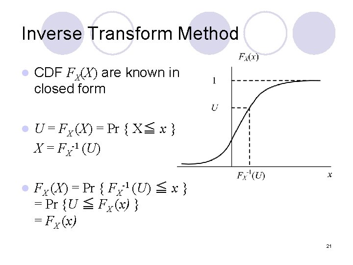
Inverse Transform Method l CDF FX(X) are known in closed form l U = FX (X) = Pr { X≦ x } X = FX-1 (U) l FX (X) = Pr { FX-1 (U) ≦ x } = Pr {U ≦ FX (x) } = FX (x) 21

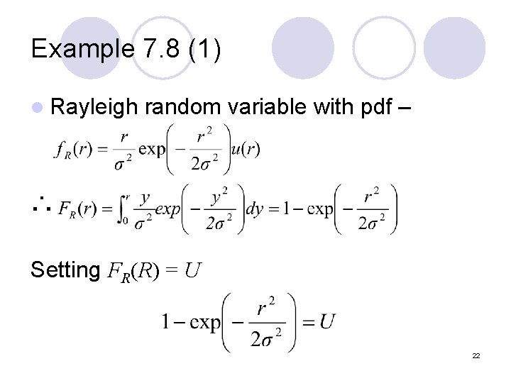
Example 7. 8 (1) l Rayleigh random variable with pdf – ∴ Setting FR(R) = U 22

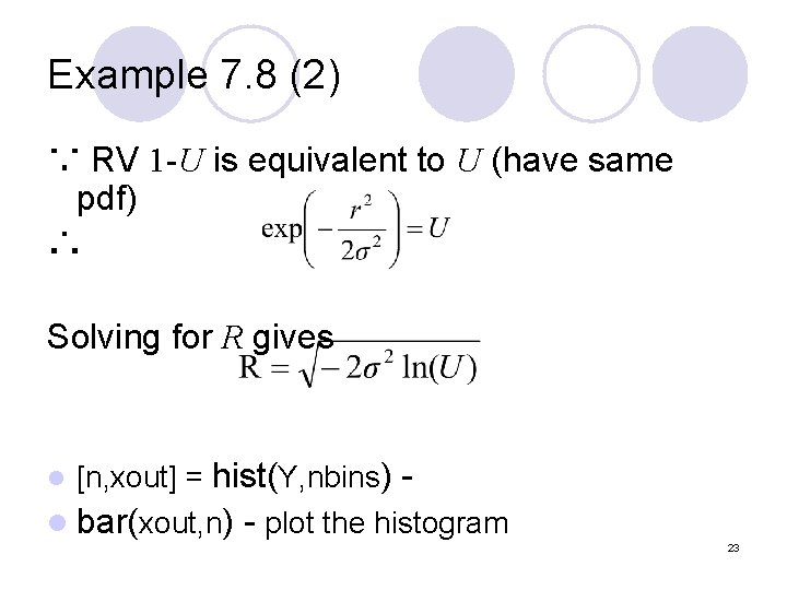
Example 7. 8 (2) ∵ RV 1 -U is equivalent to U (have same pdf) ∴ Solving for R gives l [n, xout] = hist(Y, nbins) - l bar(xout, n) - plot the histogram 23

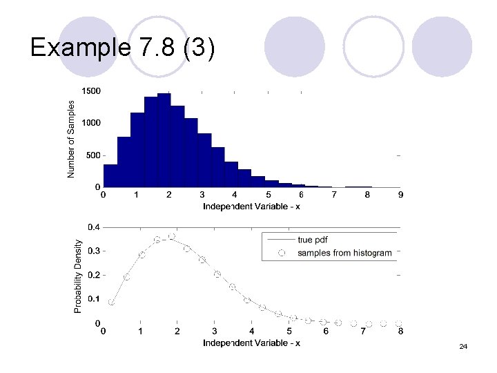
Example 7. 8 (3) 24

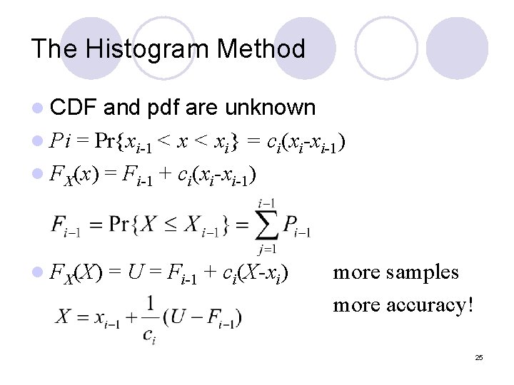
The Histogram Method l CDF and pdf are unknown l Pi = Pr{xi-1 < xi} = ci(xi-xi-1) l FX(x) = Fi-1 + ci(xi-xi-1) l FX(X) = U = Fi-1 + ci(X-xi) more samples more accuracy! 25

Rejection Methods (1) Having a target pdf l Mg. X(x) ≧ f. X(x), all x l 26

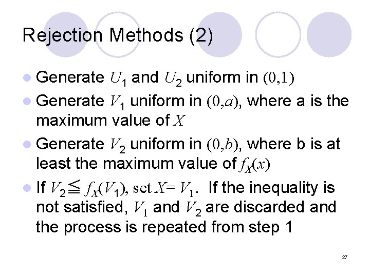
Rejection Methods (2) l Generate U 1 and U 2 uniform in (0, 1) l Generate V 1 uniform in (0, a), where a is the maximum value of X l Generate V 2 uniform in (0, b), where b is at least the maximum value of f. X(x) l If V 2≦ f. X(V 1), set X= V 1. If the inequality is not satisfied, V 1 and V 2 are discarded and the process is repeated from step 1 27

Example 7. 9 (1) 28

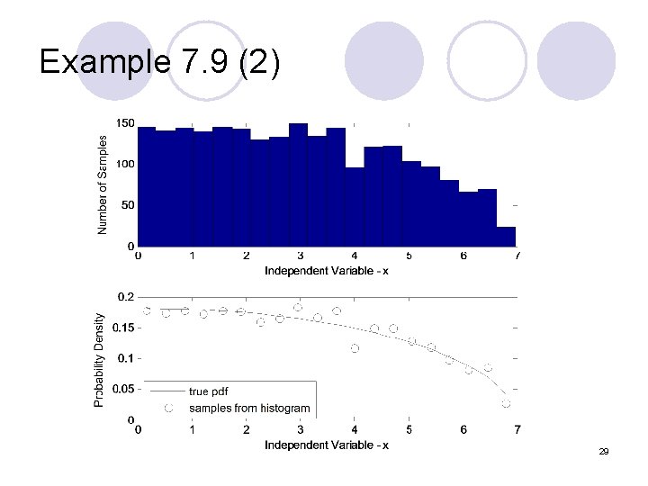
Example 7. 9 (2) 29

Generating Uncorrelated Gaussian RV l Its CDF can’t be written in closed form，so Inverse method can’t be used and rejection method are not efficient l Other techniques 1. The sum of uniform method 2. Mapping a Rayleigh to Gaussian RV 3. The polar method 30

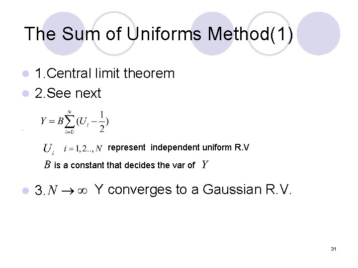
The Sum of Uniforms Method(1) 1. Central limit theorem l 2. See next l . represent independent uniform R. V is a constant that decides the var of l 3. Y converges to a Gaussian R. V. 31

The Sum of Uniforms Method(2) l Expectation and Variance We can set to any desired value l Nonzero at l 32

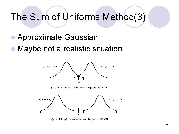
The Sum of Uniforms Method(3) l Approximate Gaussian l Maybe not a realistic situation. 33

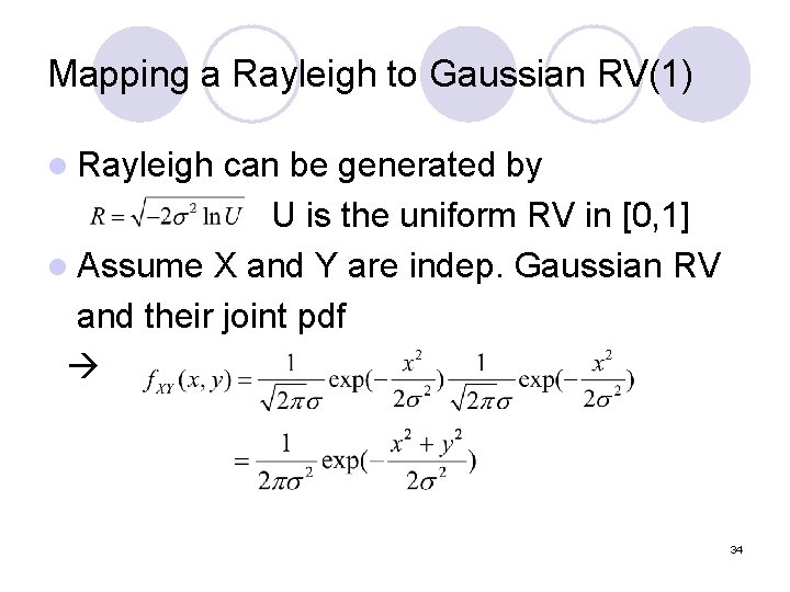
Mapping a Rayleigh to Gaussian RV(1) l Rayleigh can be generated by U is the uniform RV in [0, 1] l Assume X and Y are indep. Gaussian RV and their joint pdf 34

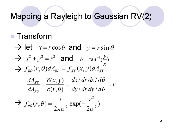
Mapping a Rayleigh to Gaussian RV(2) l Transform let and 35

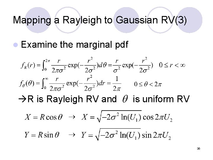
Mapping a Rayleigh to Gaussian RV(3) l Examine the marginal pdf R is Rayleigh RV and is uniform RV 36

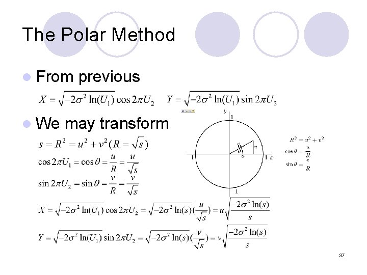
The Polar Method l From l We previous may transform 37

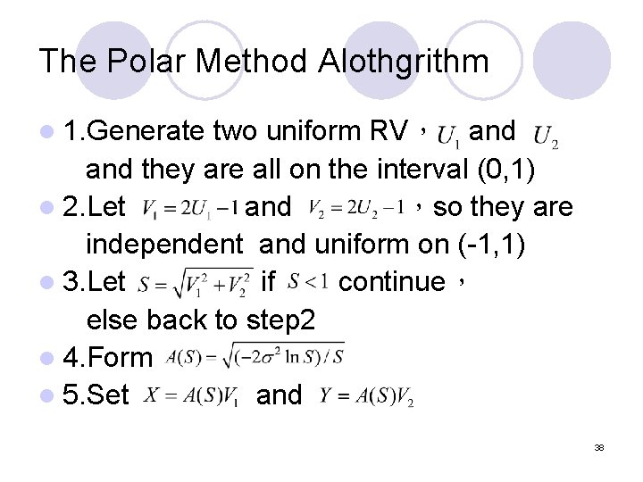
The Polar Method Alothgrithm l 1. Generate two uniform RV， and they are all on the interval (0, 1) l 2. Let and ，so they are independent and uniform on (-1, 1) l 3. Let if continue， else back to step 2 l 4. Form l 5. Set and 38

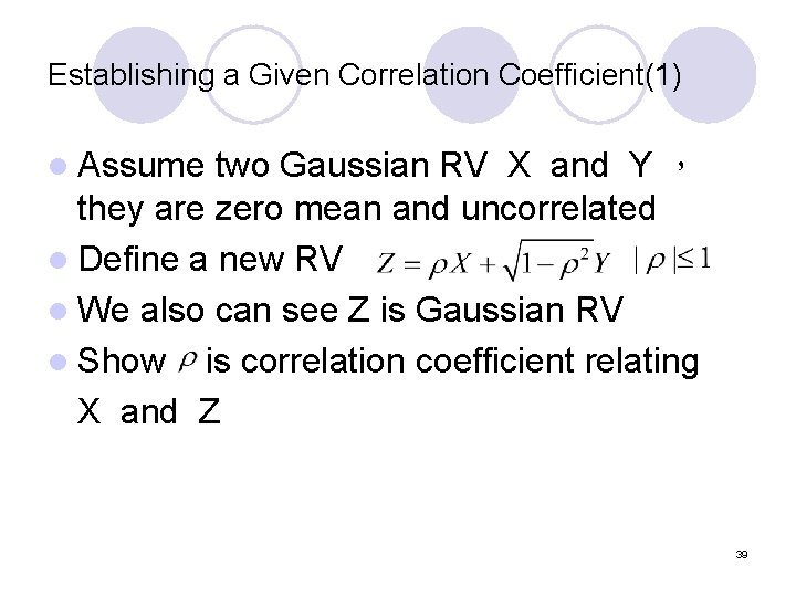
Establishing a Given Correlation Coefficient(1) l Assume two Gaussian RV X and Y ， they are zero mean and uncorrelated l Define a new RV l We also can see Z is Gaussian RV l Show is correlation coefficient relating X and Z 39

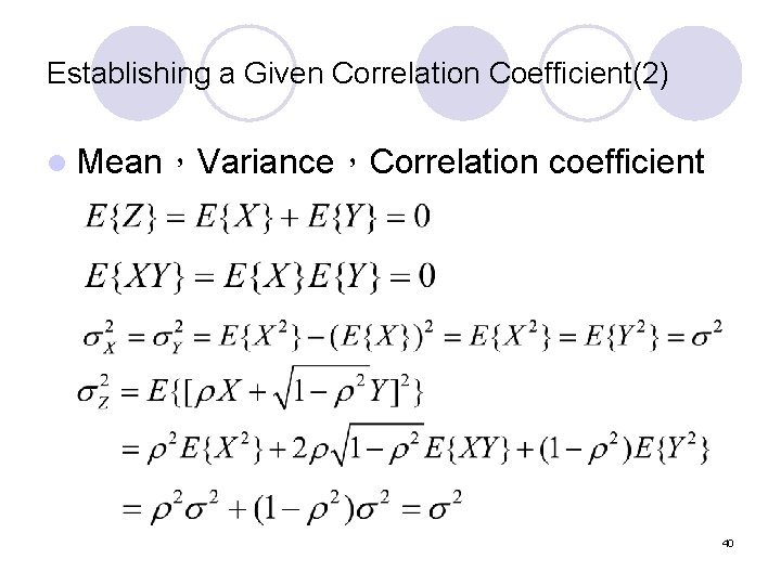
Establishing a Given Correlation Coefficient(2) l Mean，Variance，Correlation coefficient 40

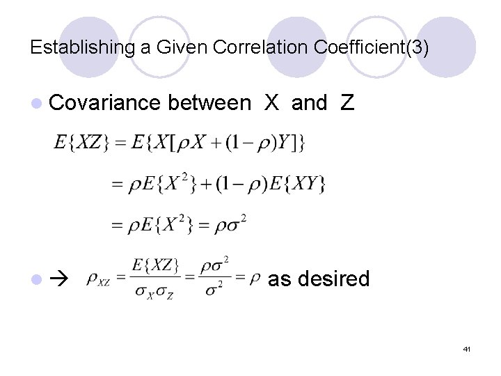
Establishing a Given Correlation Coefficient(3) l Covariance l between X and Z as desired 41

Pseudonoise(PN) Sequence Genarators l PN generator produces periodic sequence that appears to be random l Generated by algorithm using initial seed l Although not random，but can pass many tests of randomness l Unless algorithm and seed are known， the sequence is impractical to predict 42

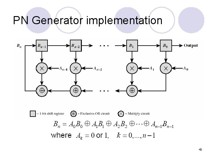
PN Generator implementation 43

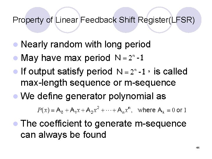
Property of Linear Feedback Shift Register(LFSR) l Nearly random with long period l May have max period l If output satisfy period ，is called max-length sequence or m-sequence l We define generator polynomial as l The coefficient to generate m-sequence can always be found 44

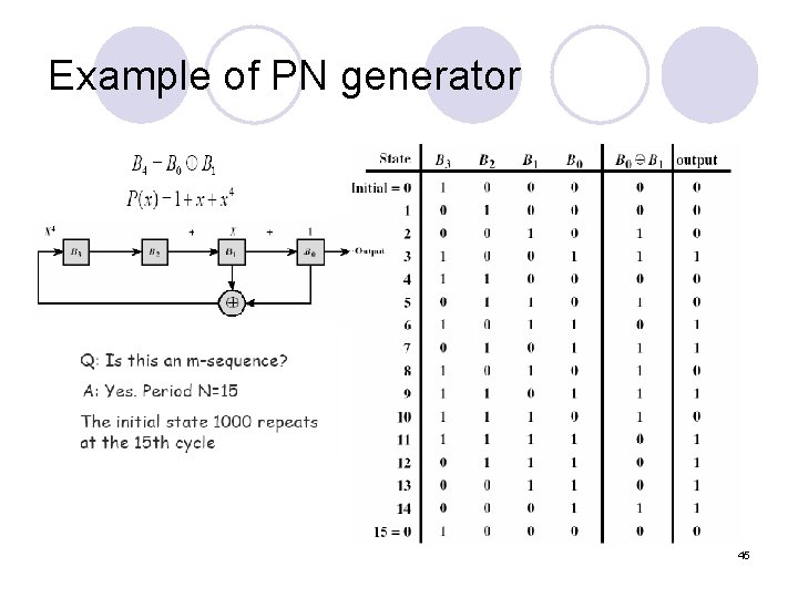
Example of PN generator 45

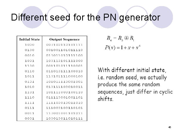
Different seed for the PN generator 46

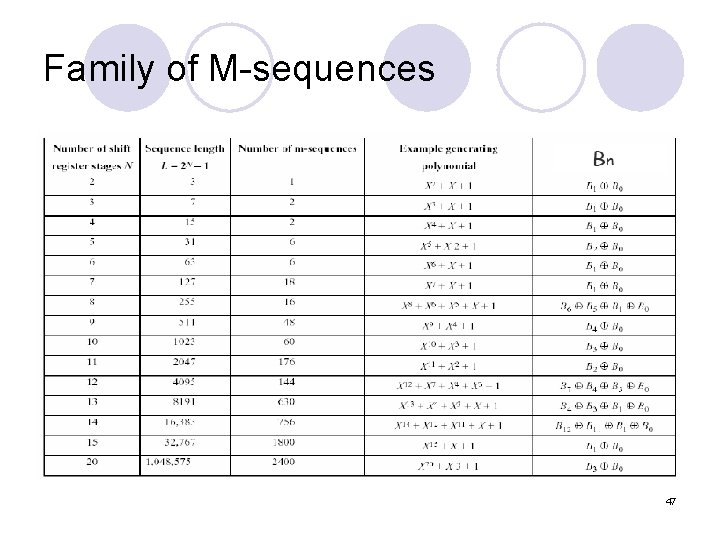
Family of M-sequences 47

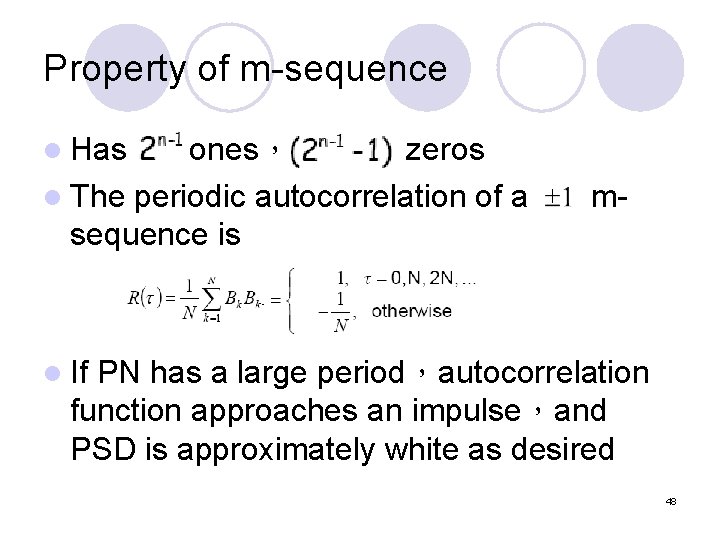
Property of m-sequence l Has ones， zeros l The periodic autocorrelation of a sequence is m- l If PN has a large period，autocorrelation function approaches an impulse，and PSD is approximately white as desired 48

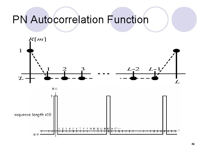
PN Autocorrelation Function 49

Signal Processing l Relationship 1. mean of input and output 2. variance of input and output 3. input-output cross-correlation 4. autocorrelation and PSD 50

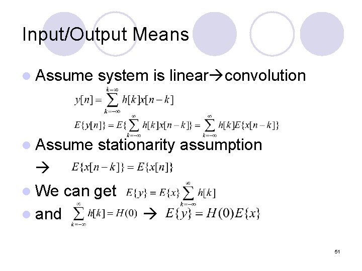
Input/Output Means l Assume system is linear convolution l Assume stationarity assumption l We can get l and 51

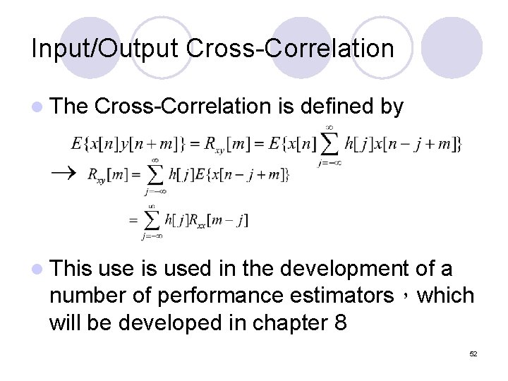
Input/Output Cross-Correlation l The Cross-Correlation is defined by l This used in the development of a number of performance estimators，which will be developed in chapter 8 52

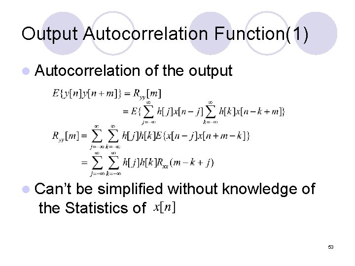
Output Autocorrelation Function(1) l Autocorrelation of the output l Can’t be simplified without knowledge of the Statistics of 53

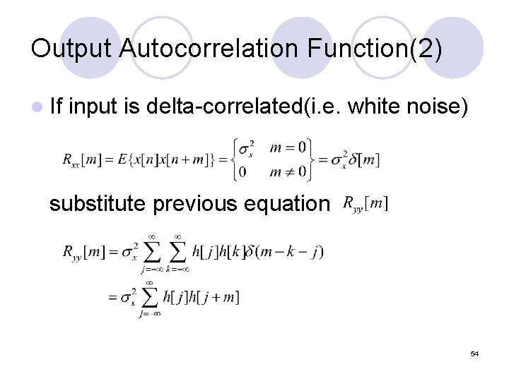
Output Autocorrelation Function(2) l If input is delta-correlated(i. e. white noise) substitute previous equation 54

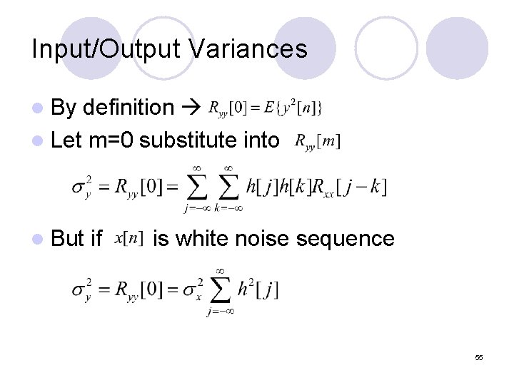
Input/Output Variances l By definition l Let m=0 substitute into l But if is white noise sequence 55

The End Thanks for listening 56