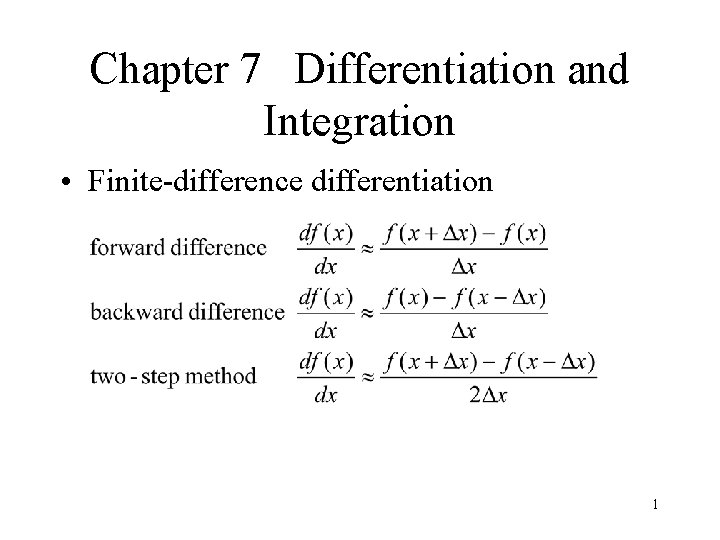
Chapter 7 Differentiation and Integration Finitedifference differentiation 1

Chapter 7 Differentiation and Integration • Finite-difference differentiation 1

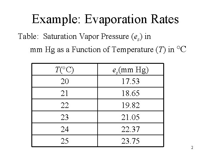
Example: Evaporation Rates Table: Saturation Vapor Pressure (es) in mm Hg as a Function of Temperature (T) in °C T(°C) 20 21 22 23 24 25 es(mm Hg) 17. 53 18. 65 19. 82 21. 05 22. 37 23. 75 2

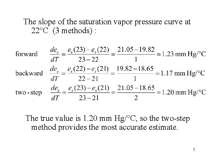
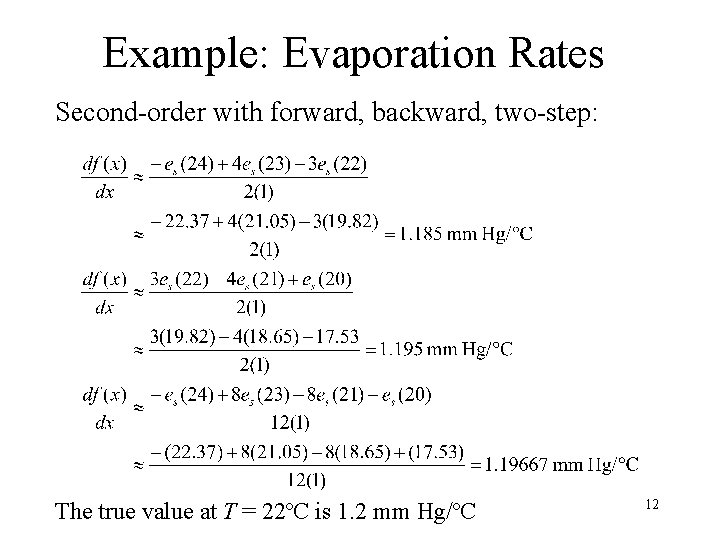
The slope of the saturation vapor pressure curve at 22°C (3 methods) : The true value is 1. 20 mm Hg/°C, so the two-step method provides the most accurate estimate. 3

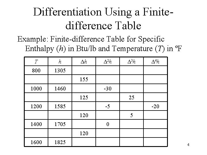
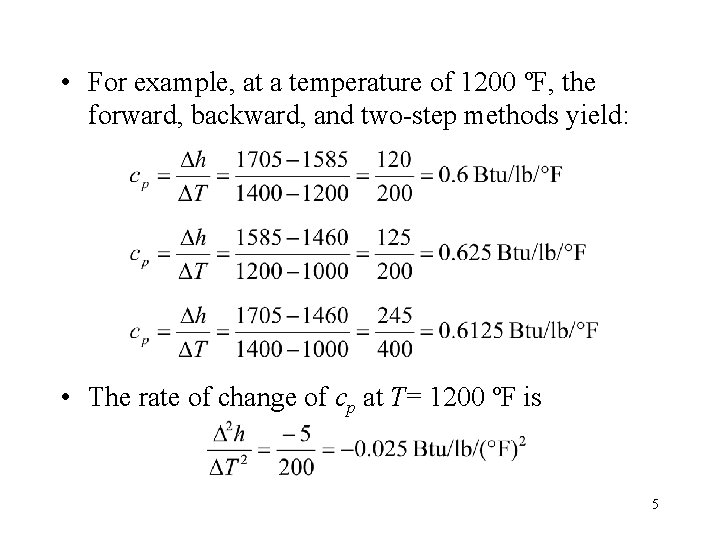
Differentiation Using a Finitedifference Table Example: Finite-difference Table for Specific Enthalpy (h) in Btu/lb and Temperature (T) in ºF T h 800 1305 Δh Δ 2 h Δ 3 h Δ 4 h 155 1000 1460 -30 125 1200 1585 25 -5 120 1400 1705 -20 5 0 120 1600 1825 4

• For example, at a temperature of 1200 ºF, the forward, backward, and two-step methods yield: • The rate of change of cp at T= 1200 ºF is 5

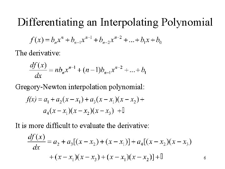
Differentiating an Interpolating Polynomial The derivative: Gregory-Newton interpolation polynomial: It is more difficult to evaluate the derivative: 6

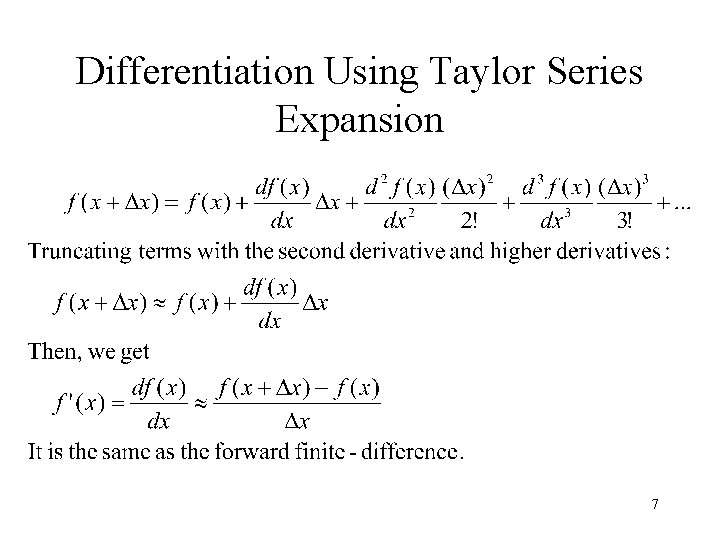
Differentiation Using Taylor Series Expansion 7

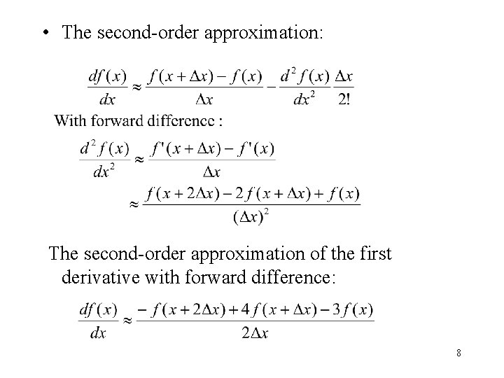
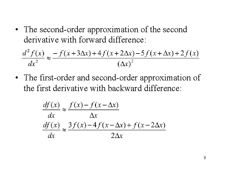
• The second-order approximation: The second-order approximation of the first derivative with forward difference: 8

• The second-order approximation of the second derivative with forward difference: • The first-order and second-order approximation of the first derivative with backward difference: 9

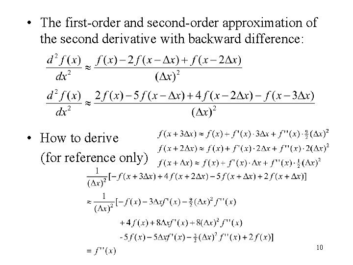
• The first-order and second-order approximation of the second derivative with backward difference: • How to derive (for reference only) 10

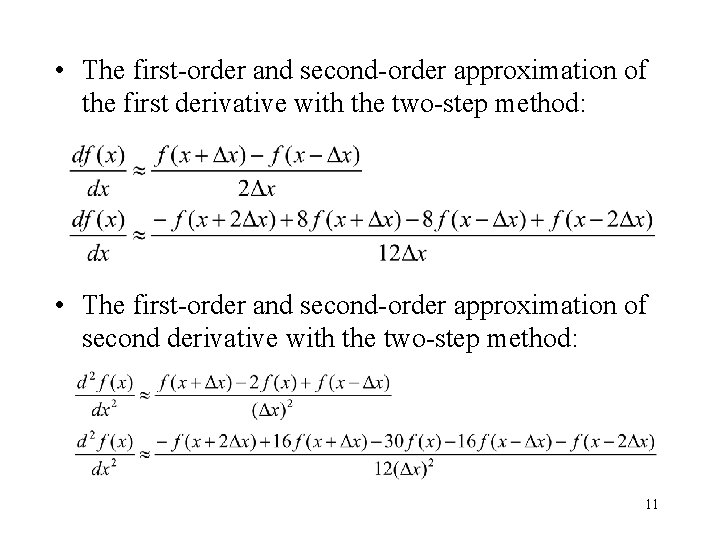
• The first-order and second-order approximation of the first derivative with the two-step method: • The first-order and second-order approximation of second derivative with the two-step method: 11

Example: Evaporation Rates Second-order with forward, backward, two-step: The true value at T = 22ºC is 1. 2 mm Hg/ºC 12

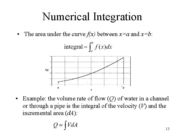
Numerical Integration • The area under the curve f(x) between x=a and x=b: • Example: the volume rate of flow (Q) of water in a channel or through a pipe is the integral of the velocity (V) and the incremental area (d. A): 13

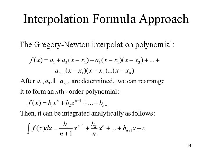
Interpolation Formula Approach The Gregory-Newton interpolation polynomial: 14

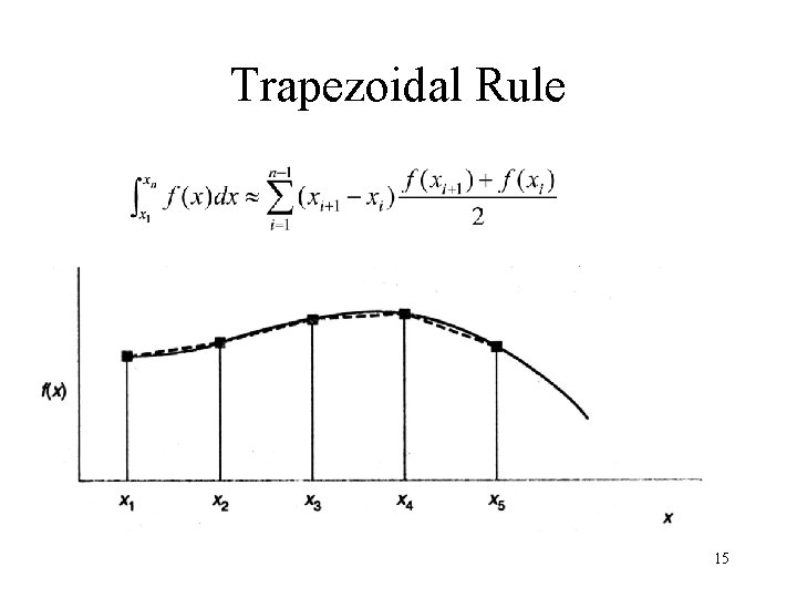
Trapezoidal Rule 15

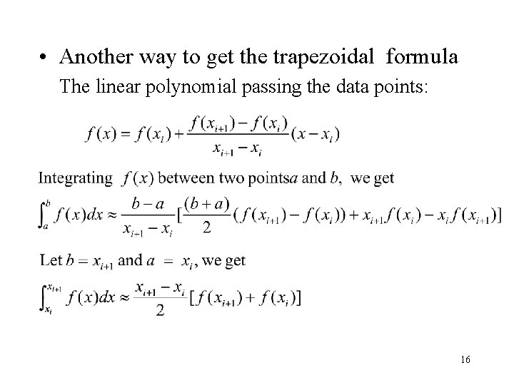
• Another way to get the trapezoidal formula The linear polynomial passing the data points: 16

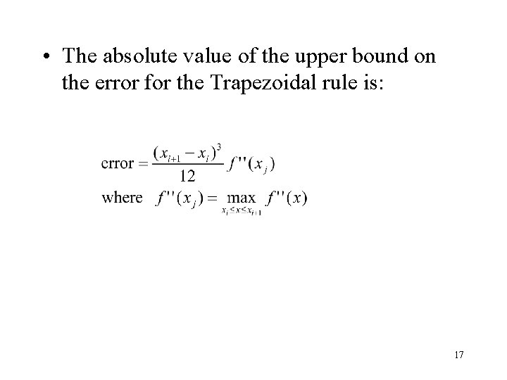
• The absolute value of the upper bound on the error for the Trapezoidal rule is: 17

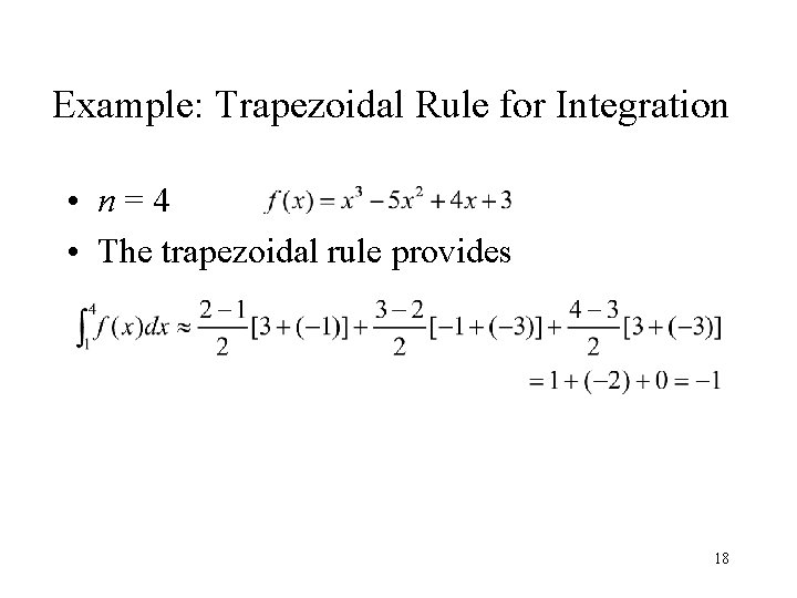
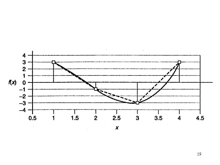
Example: Trapezoidal Rule for Integration • n=4 • The trapezoidal rule provides 18

19

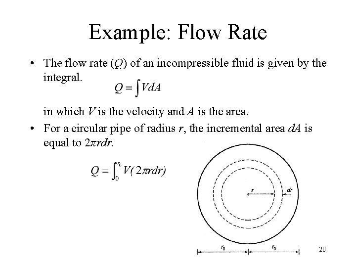
Example: Flow Rate • The flow rate (Q) of an incompressible fluid is given by the integral. in which V is the velocity and A is the area. • For a circular pipe of radius r, the incremental area d. A is equal to 2πrdr. 20

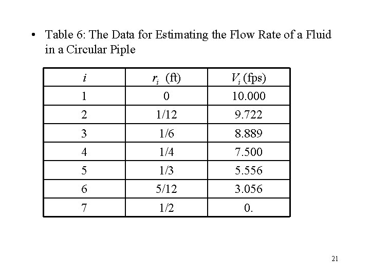
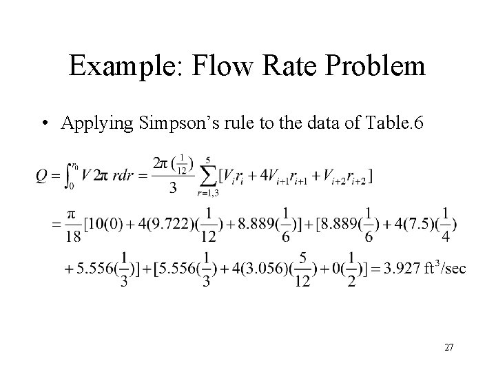
• Table 6: The Data for Estimating the Flow Rate of a Fluid in a Circular Piple i ri (ft) Vi (fps) 1 0 10. 000 2 1/12 9. 722 3 1/6 8. 889 4 1/4 7. 500 5 1/3 5. 556 6 5/12 3. 056 7 1/2 0. 21

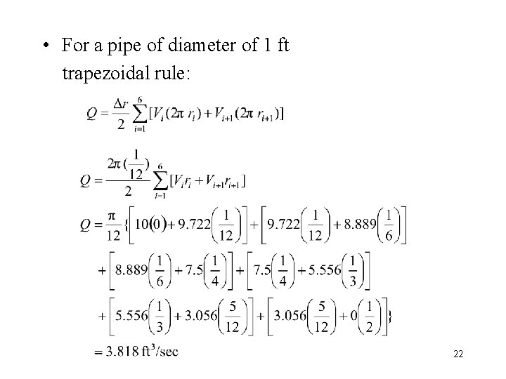
• For a pipe of diameter of 1 ft trapezoidal rule: 22

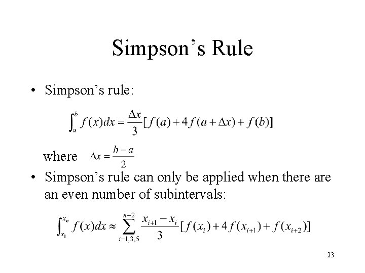
Simpson’s Rule • Simpson’s rule: where • Simpson’s rule can only be applied when there an even number of subintervals: 23

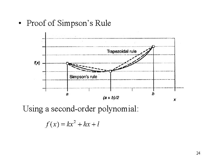
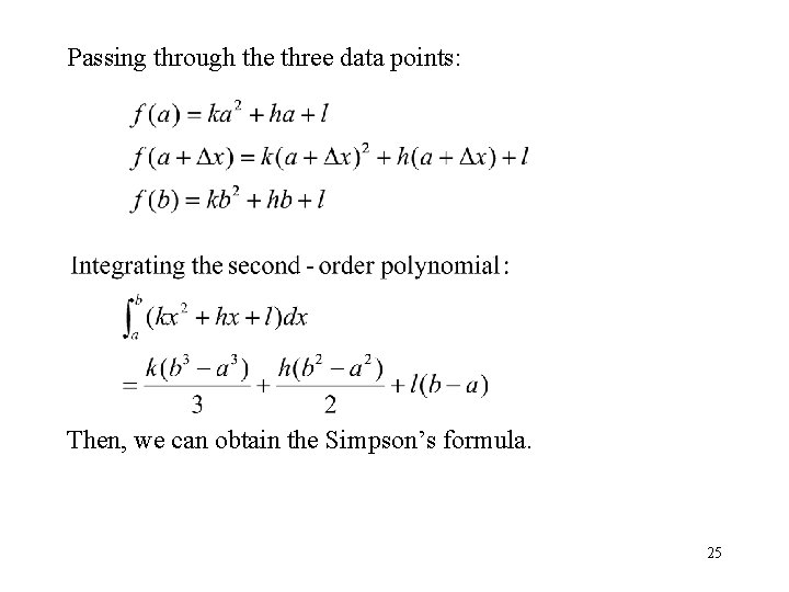
• Proof of Simpson’s Rule Using a second-order polynomial: 24

Passing through the three data points: Then, we can obtain the Simpson’s formula. 25

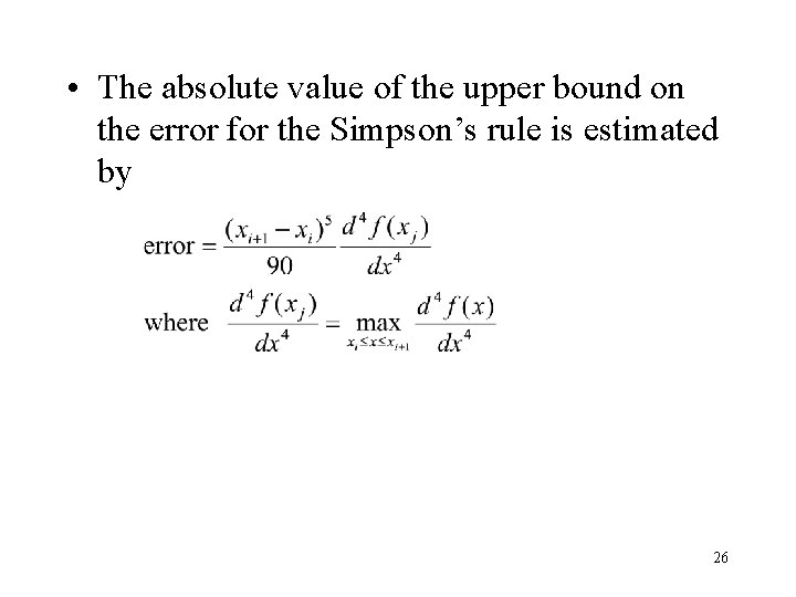
• The absolute value of the upper bound on the error for the Simpson’s rule is estimated by 26

Example: Flow Rate Problem • Applying Simpson’s rule to the data of Table. 6 27

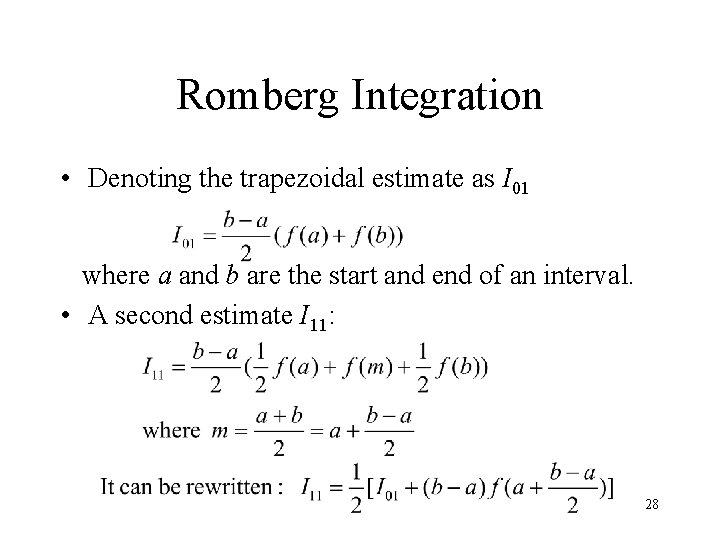
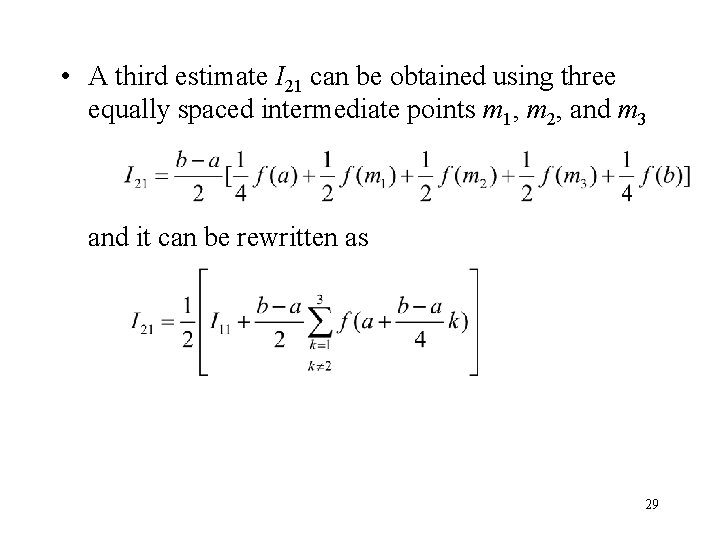
Romberg Integration • Denoting the trapezoidal estimate as I 01 where a and b are the start and end of an interval. • A second estimate I 11: 28

• A third estimate I 21 can be obtained using three equally spaced intermediate points m 1, m 2, and m 3 and it can be rewritten as 29

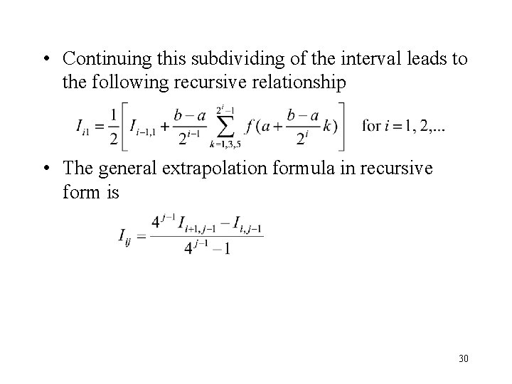
• Continuing this subdividing of the interval leads to the following recursive relationship • The general extrapolation formula in recursive form is 30

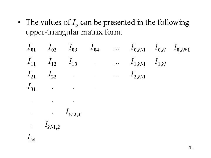
• The values of Iij can be presented in the following upper-triangular matrix form: I 01 I 02 I 03 I 04 … I 0, N-1 I 0, N I 11 I 12 I 13 . … I 1, N-1 I 1, N I 21 I 22 . . … I 2, N-1 I 31 . . . . IN-2, 3 . IN-1, 2 I 0, N+1 IN 1 31

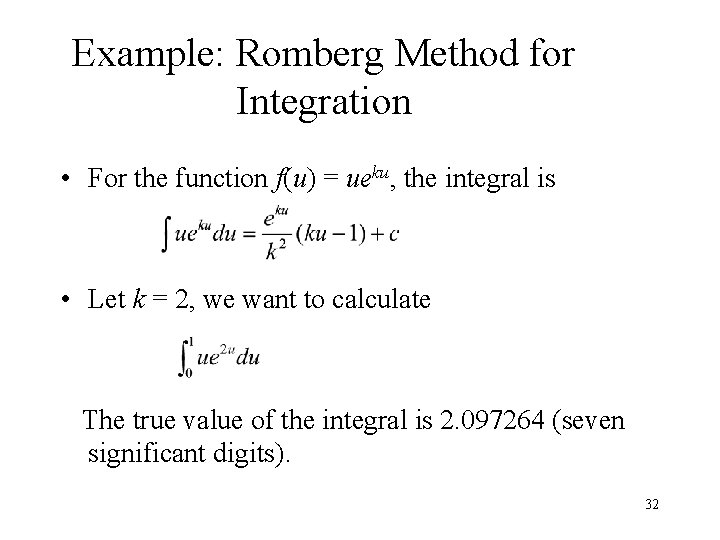
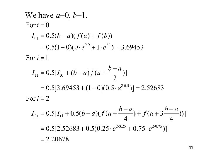
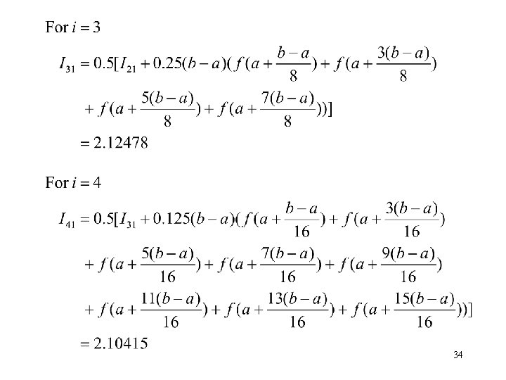
Example: Romberg Method for Integration • For the function f(u) = ueku, the integral is • Let k = 2, we want to calculate The true value of the integral is 2. 097264 (seven significant digits). 32

We have a=0, b=1. 33

34

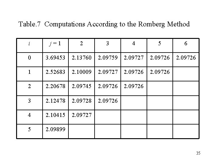
Table. 7 Computations According to the Romberg Method i j=1 2 3 4 5 6 0 3. 69453 2. 13760 2. 09759 2. 09727 2. 09726 1 2. 52683 2. 10009 2. 09727 2. 09726 2 2. 20678 2. 09745 2. 09726 3 2. 12478 2. 09726 4 2. 10415 2. 09727 5 2. 09899 35

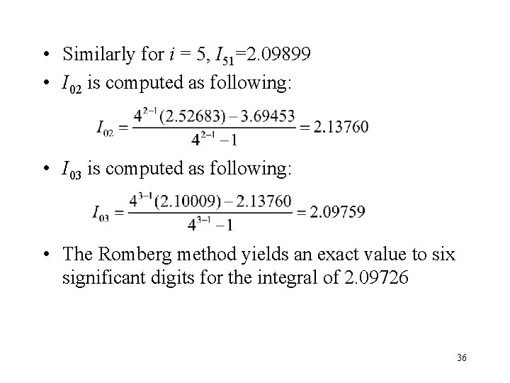
• Similarly for i = 5, I 51=2. 09899 • I 02 is computed as following: • I 03 is computed as following: • The Romberg method yields an exact value to six significant digits for the integral of 2. 09726 36