CHAPTER 7 DESCRIBING AND PRESENTING DATA Descriptive Statistics

CHAPTER 7 DESCRIBING AND PRESENTING DATA
Descriptive Statistics We use descriptive statistics in two ways: 1. They provide a description of our sample by summarizing and organizing our data. E. g. variables such as gender, age, income, no. of employees in organization, sales, etc. 2. They provide statistics such as averages and spreads of scores of variables for the sample which will be later used as the estimates of the parameters of the population when we conduct inferential statistics.
DESCRIPTIVE STATISTICS ORGANIZING THE DATA They often involve calculating as well as producing graphical displays of (inter alia) – frequencies of different occurrences, – central location of a distribution, – spread of a distribution, – shape of a distribution
Four Common Descriptive ‘Summary' Measures: • The distribution of frequencies • Measures of the central tendency of the data • Measures of dispersion, spread or variability • Skewness or normality of spread
Measures of Central Tendency ‘Measures of central tendency’ are also referred to as ‘averages’. The purpose of a measure of central tendency is to provide a single value which summarizes a variable. There are three commonly used measures of central tendency. These are:
MEASURES OF CENTRAL TENDENCY • The Mode – The most frequently occurring score value • The Median – The middle value when scores are placed in rank order • The Mean – the sum of all the scores divided by the number of scores, i. e. the arithmetical average
Measures of Central Tendency: Mode: the most commonly occurring observation/value/case. The mode (or modal class) can be calculated for nominal, ordinal, interval, or ratio scale data. e. g. 2, 2, 2, 3, 4, 5, 1000. Mode = 2 With a variable measured on interval or ratio scales, there may be no two values which are identical. In this case a ‘modal class’ may be calculated by first grouping your cases into ranges (e. g. 0 -18 years, 19 -29 years, 30 -39 years, etc) and determining the category with the largest number of cases (the ‘modal class’).
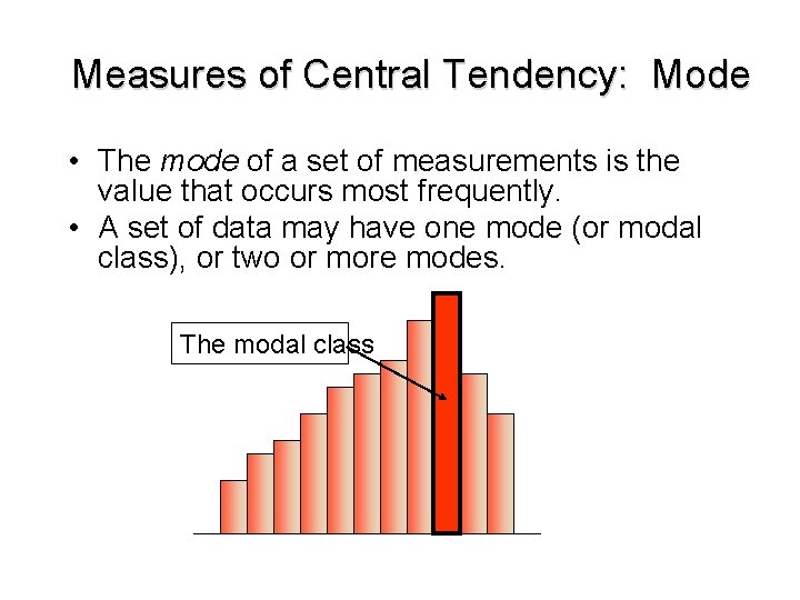
Measures of Central Tendency: Mode • The mode of a set of measurements is the value that occurs most frequently. • A set of data may have one mode (or modal class), or two or more modes. The modal class
Measures of Central Tendency: Median: the middle value in an ordered array. The median can be calculated for ordinal, interval, or ratio scale data. Used instead of mean for skewed distributions like that below. e. g. 2, 2, 2, 3, 4, 5, 1000. Median = 3
Measures of Central Tendency: Arithmetic Mean: measure of the central data point (the sum of the measures in the set divided by the number of scores in the set). Common name is ‘average’ The arithmetic mean can be calculated for interval or ratio scale data. e. g. 2, 2, 2, 3, 4, 5, 1000. Mean = 145. 4
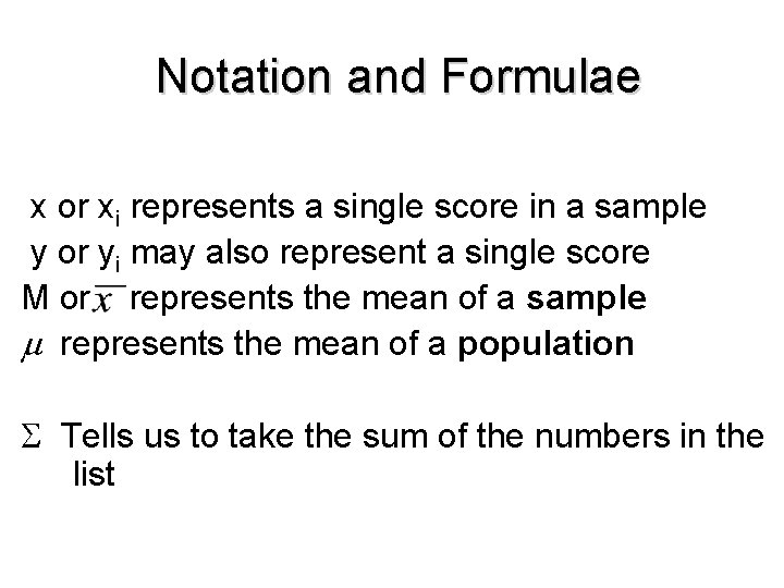
Notation and Formulae x or xi represents a single score in a sample y or yi may also represent a single score M or represents the mean of a sample represents the mean of a population Tells us to take the sum of the numbers in the list
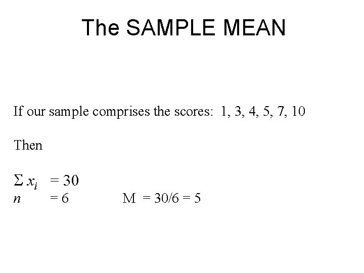
The SAMPLE MEAN If our sample comprises the scores: 1, 3, 4, 5, 7, 10 Then xi = 30 n =6 M = 30/6 = 5
The Mean • Characteristics: – determined by the value of every score – amenable to arithmetic and algebraic manipulations • Problems with the mean: – when the distribution is very skewed it provides an inaccurate picture of where the central values are – when the data are qualitative in character it cannot be calculated
Central Tendency and Levels of Measurement • nominal scale: – the mode is the only legitimate statistic to use. • ordinal scale: – median preferred over the mean which could be distorted by an extreme score • interval and ratio scales (grouped together as Scale level in SPSS): – the mean is the recommended measure of central tendency, median & mode may also be reported for these types of scales
MEASURES OF VARIABILITY • Measures of central tendency do not provide information about the distribution of scores for a variable. • Questions unanswered are: How typical is the average value of all the measurements in the data set? or How spread out are the measurements around the average value?
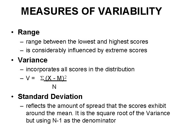
MEASURES OF VARIABILITY • Range – range between the lowest and highest scores – is considerably influenced by extreme scores • Variance – incorporates all scores in the distribution – V = (X - M)2 N • Standard Deviation – reflects the amount of spread that the scores exhibit around the mean. It is the square root of the Variance but using N-1 as the denominator
Measures of Variability: Range – The range of a set of measurements is the difference between the largest and smallest measurements. – Its major advantage is the ease with which it can be computed. – Its major shortcoming is that it is influenced totally by the values of the smallest and largest scores with no information on the spread of values between the end points.
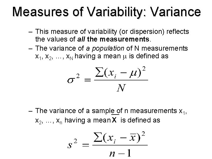
Measures of Variability: Variance – This measure of variability (or dispersion) reflects the values of all the measurements. – The variance of a population of N measurements x 1, x 2, …, x. N having a mean m is defined as – The variance of a sample of n measurements x 1, x 2, …, xn having a mean is defined as
Standard Deviation – The standard deviation of a set of values is the square root of the variance of the measurements. - The standard deviation is more commonly reported than the variance. - It is calculated from all the values in a data set, representing the dispersal round the mean outward in each direction.
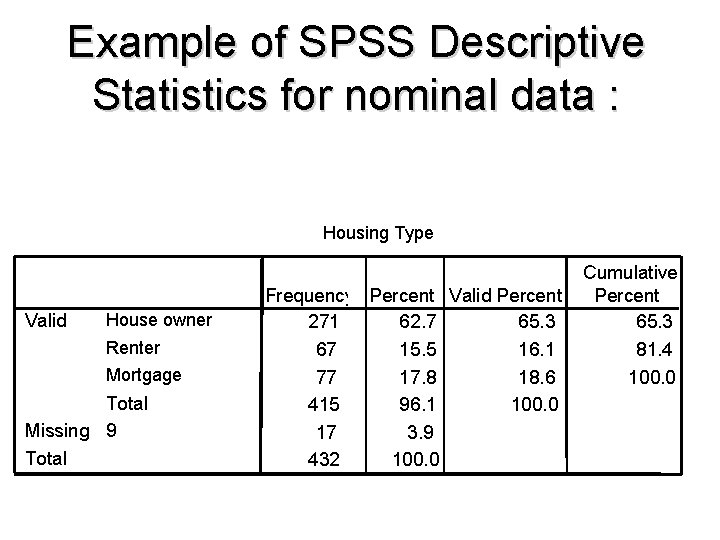
Example of SPSS Descriptive Statistics for nominal data : Housing Type Valid House owner Renter Mortgage Total Missing 9 Total Frequency Percent Valid Percent 271 62. 7 65. 3 67 15. 5 16. 1 77 17. 8 18. 6 415 96. 1 100. 0 17 3. 9 432 100. 0 Cumulative Percent 65. 3 81. 4 100. 0
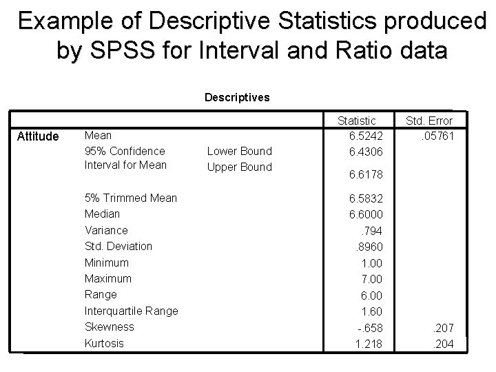
Example of Descriptive Statistics produced by SPSS for Interval and Ratio data Descriptives Attitude Mean 95% Confidence Interval for Mean 5% Trimmed Mean Median Variance Std. Deviation Minimum Maximum Range Interquartile Range Skewness Kurtosis Lower Bound Upper Bound Statistic 6. 5242 6. 4306 Std. Error. 05761 6. 6178 6. 5832 6. 6000. 794. 8960 1. 00 7. 00 6. 00 1. 60 -. 658 1. 218 . 207. 204
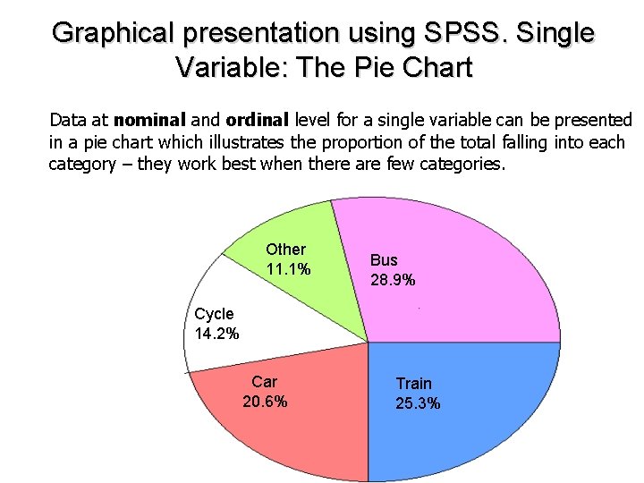
Graphical presentation using SPSS. Single Variable: The Pie Chart Data at nominal and ordinal level for a single variable can be presented in a pie chart which illustrates the proportion of the total falling into each category – they work best when there are few categories. Other 11. 1% Bus 28. 9% Cycle 14. 2% Car 20. 6% Train 25. 3%
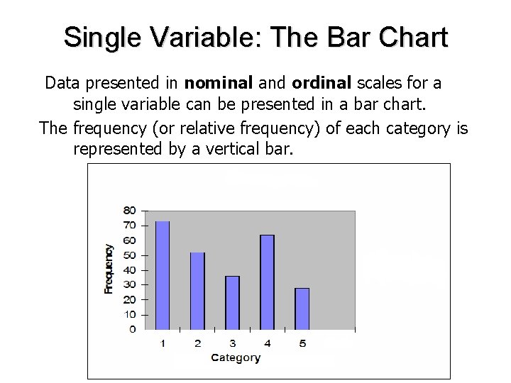
Single Variable: The Bar Chart Data presented in nominal and ordinal scales for a single variable can be presented in a bar chart. The frequency (or relative frequency) of each category is represented by a vertical bar.
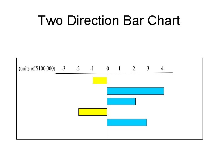
Two Direction Bar Chart
Single Variable: Stem and Leaf Displays The stem-and-leaf diagram shows the value of each of the original observations. No information is lost from the raw data to the graphical presentation. Stem-and-leaf displays are used with interval and ratio scale data. Useful in detecting outliers or erroneous out of range data
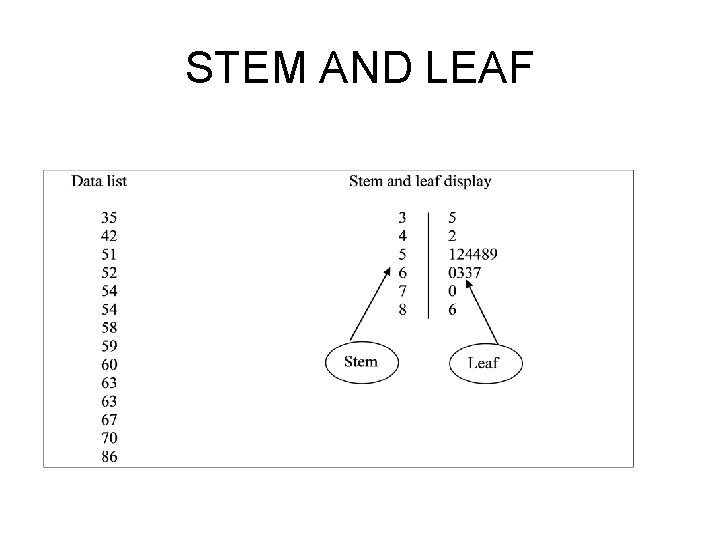
STEM AND LEAF
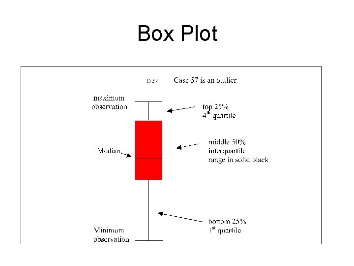
Box Plot
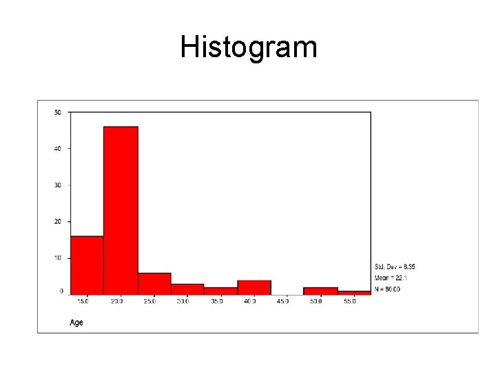
Histogram
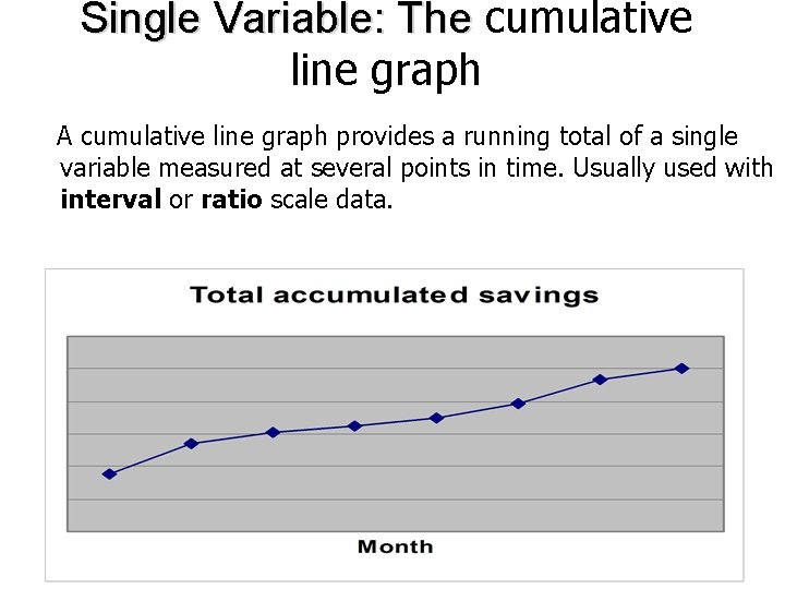
Single Variable: The cumulative line graph A cumulative line graph provides a running total of a single variable measured at several points in time. Usually used with interval or ratio scale data. Other 11. 1%
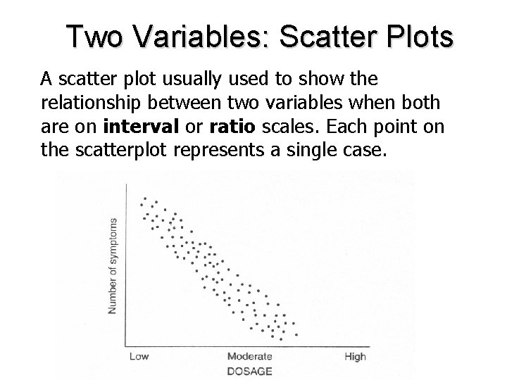
Two Variables: Scatter Plots A scatter plot usually used to show the relationship between two variables when both are on interval or ratio scales. Each point on the scatterplot represents a single case.
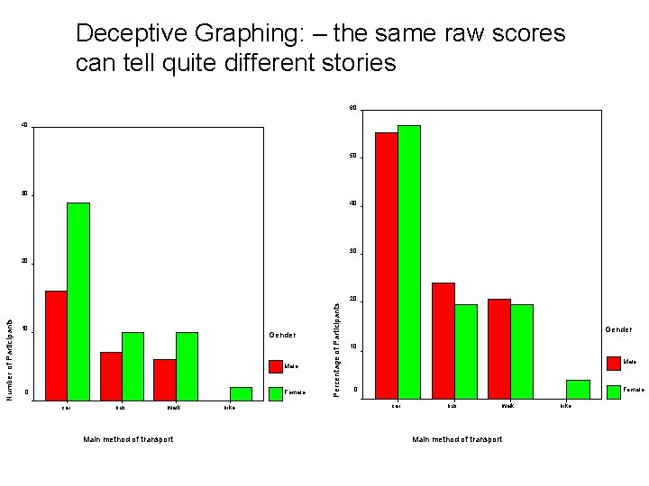
Deceptive Graphing: – the same raw scores can tell quite different stories 60 40 50 30 40 30 20 10 Gender Male 0 Female car bus walk Main method of transport bike Percentage of Participants Number of Participants 20 Gender 10 Male 0 Female car bus walk Main method of transport bike
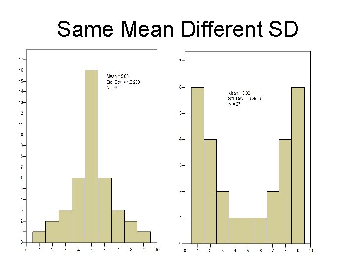
Same Mean Different SD
- Slides: 32