Chapter 7 Data Matching PRINCIPLES OF DATA INTEGRATION

Chapter 7: Data Matching PRINCIPLES OF DATA INTEGRATION ANHAI DOAN ALON HALEVY ZACHARY IVES

Data Matching

Introduction § Data matching: find structured data items that refer to the same real-world entity § entities may be represented by tuples, XML elements, or RDF triples, not by strings as in string matching § e. g. , (David Smith, 608 -245 -4367, Madison WI) vs (D. M. Smith, 245 -4367, Madison WI) § A critical problem in data science § Also known as entity matching, record linkage, entity resolution, deduplication, etc. 3

Outline § § § Problem definition Rule-based matching Learning- based matching Matching by clustering Scaling up data matching 4

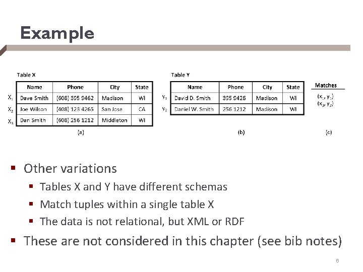
Problem Definition § Given two relational tables X and Y with identical schemas § assume each tuple in X and Y describes an entity (e. g. , person) § We say tuple x 2 X matches tuple y 2 Y if they refer to the same real-world entity § (x, y) is called a match § Goal: find all matches between X and Y 5

Example § Other variations § Tables X and Y have different schemas § Match tuples within a single table X § The data is not relational, but XML or RDF § These are not considered in this chapter (see bib notes) 6

Why is This Different than String Matching? § In theory, can treat each tuple as a string by concatenating the fields, then apply string matching techniques § But doing so makes it hard to apply sophisticated techniques and domain-specific knowledge § E. g. , consider matching tuples that describe persons § suppose we know that in this domain two tuples match if the names and phone match exactly § this knowledge is hard to encode if we use string matching § so it is better to keep the fields apart 7

Challenges § Same as in string matching § How to match accurately? § difficult due to variations in formatting conventions, use of abbreviations, shortening, different naming conventions, omissions, nicknames, and errors in data § several common approaches: rule-based, learning-based, clustering, probabilistic, collective § How to scale up to large data sets § again many approaches have been developed, as we will discuss 8

Outline § § § § Problem definition Rule-based matching Learning- based matching Matching by clustering Probabilistic approaches to matching Collective matching Scaling up data matching 9

Rule-based Matching § The developer writes rules that specify when two tuples match § typically after examining many matching and non-matching tuple pairs, using a development set of tuple pairs § rules are then tested and refined, using the same development set or a test set § Many types of rules exist, we will consider § linearly weighted combination of individual similarity scores § logistic regression combination § more complex rules 10

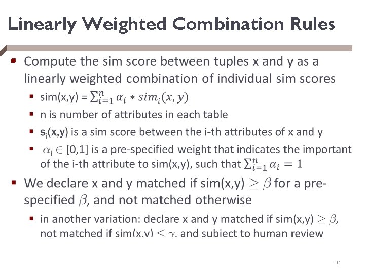
Linearly Weighted Combination Rules § 11

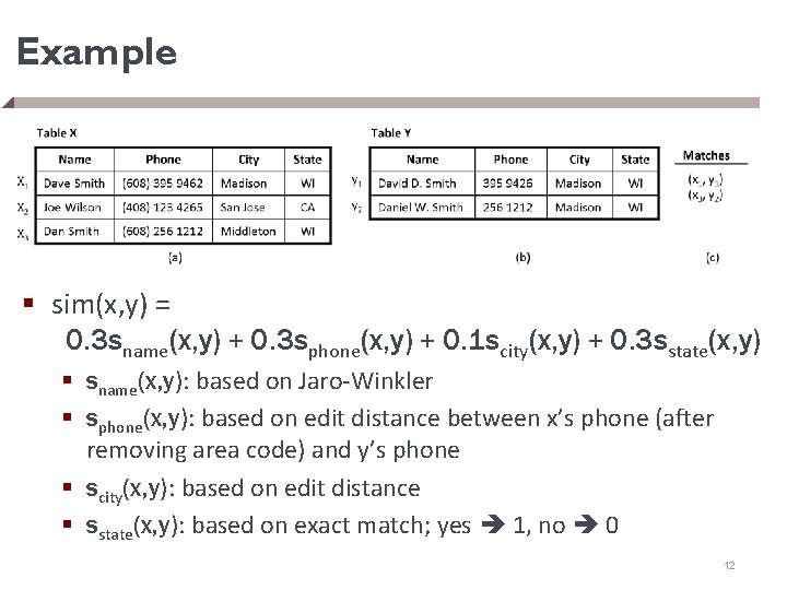
Example § sim(x, y) = 0. 3 sname(x, y) + 0. 3 sphone(x, y) + 0. 1 scity(x, y) + 0. 3 sstate(x, y) § sname(x, y): based on Jaro-Winkler § sphone(x, y): based on edit distance between x’s phone (after removing area code) and y’s phone § scity(x, y): based on edit distance § sstate(x, y): based on exact match; yes 1, no 0 12

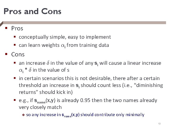
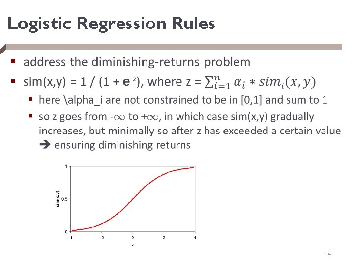
Pros and Cons § Pros § conceptually simple, easy to implement § can learn weights ®i from training data § Cons § an increase ± in the value of any si will cause a linear increase ®i * ± in the value of s § in certain scenarios this is not desirable, there after a certain threshold an increase in si should count less (i. e. , “diminishing returns” should kick in) § e. g. , if sname(x, y) is already 0. 95 then the two names already very closely match v so any increase in sname(x, y) should contribute only minimally 13

Logistic Regression Rules § 14

Logistic Regression Rules § Are also very useful in situations where § there are many “signals” (e. g. , 10 -20) that can contribute to whether two tuples match § we don’t need all of these signals to “fire” in order to conclude that the tuples match § as long as a reasonable number of them fire, we have sufficient confidence § Logistic regression is a natural fit for such cases § Hence is quite popular as a first matching method to try 15

More Complex Rules § Appropriate when we want to encode more complex matching knowledge § e. g. , two persons match if names match approximately and either phones match exactly or addresses match exactly 1. If sname(x, y) < 0. 8 then return “not matched” 2. Otherwise if ephone(x, y) = true then return “matched” 3. Otherwise if ecity(x, y) = true and estate(x, y) = true then return “matched” 4. Otherwise return “not matched” 16

Pros and Cons of Rule-Based Approaches § Pros § easy to start, conceptually relatively easy to understand, implement, debug § typically run fast § can encode complex matching knowledge § Cons § § can be labor intensive, it takes a lot of time to write good rules can be difficult to set appropriate weights in certain cases it is not even clear how to write rules learning-based approaches address these issues 17

Outline § § § § Problem definition Rule-based matching Learning- based matching Matching by clustering Probabilistic approaches to matching Collective matching Scaling up data matching 18

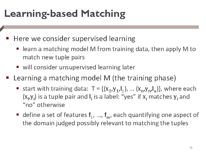
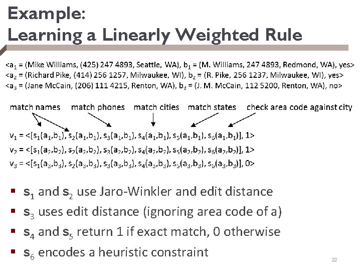
Learning-based Matching § Here we consider supervised learning § learn a matching model M from training data, then apply M to match new tuple pairs § will consider unsupervised learning later § Learning a matching model M (the training phase) § start with training data: T = {(x 1, y 1, l 1), … (xn, yn, ln)}, where each (xi, yi) is a tuple pair and li is a label: “yes” if xi matches yi and “no” otherwise § define a set of features f 1, …, fm, each quantifying one aspect of the domain judged possibly relevant to matching the tuples 19

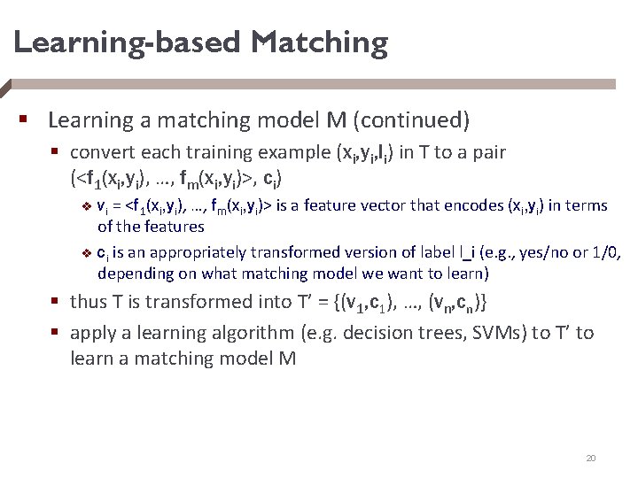
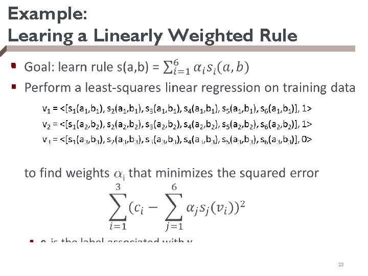
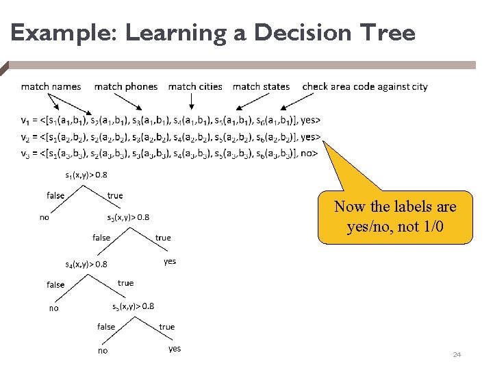
Learning-based Matching § Learning a matching model M (continued) § convert each training example (xi, yi, li) in T to a pair (<f 1(xi, yi), …, fm(xi, yi)>, ci) v vi = <f 1(xi, yi), …, fm(xi, yi)> is a feature vector that encodes (xi, yi) in terms of the features v ci is an appropriately transformed version of label l_i (e. g. , yes/no or 1/0, depending on what matching model we want to learn) § thus T is transformed into T’ = {(v 1, c 1), …, (vn, cn)} § apply a learning algorithm (e. g. decision trees, SVMs) to T’ to learn a matching model M 20

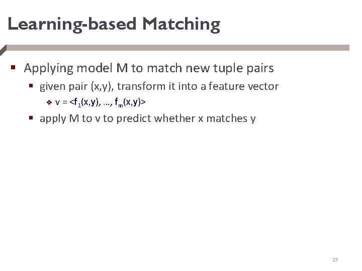
Learning-based Matching § Applying model M to match new tuple pairs § given pair (x, y), transform it into a feature vector v v = <f 1(x, y), …, fm(x, y)> § apply M to v to predict whether x matches y 21

Example: Learning a Linearly Weighted Rule § § s 1 and s 2 use Jaro-Winkler and edit distance s 3 uses edit distance (ignoring area code of a) s 4 and s 5 return 1 if exact match, 0 otherwise s 6 encodes a heuristic constraint 22

Example: Learing a Linearly Weighted Rule § 23

Example: Learning a Decision Tree Now the labels are yes/no, not 1/0 24

The Pros and Cons of Learning-based Approach § Pros compared to rule-based approaches § in rule-based approaches must manually decide if a particular feature is useful labor intensive and limit the number of features we can consider § learning-based ones can automatically examine a large number of features § learning-based approaches can construct very complex “rules” § Cons § still require training examples, in many cases a large number of them, which can be hard to obtain § clustering addresses this problem 25

Outline § § § § Problem definition Rule-based matching Learning- based matching Matching by clustering Probabilistic approaches to matching Collective matching Scaling up data matching 26

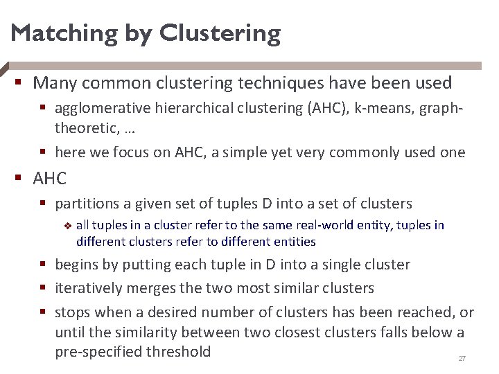
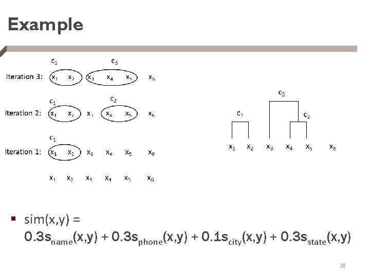
Matching by Clustering § Many common clustering techniques have been used § agglomerative hierarchical clustering (AHC), k-means, graphtheoretic, … § here we focus on AHC, a simple yet very commonly used one § AHC § partitions a given set of tuples D into a set of clusters v all tuples in a cluster refer to the same real-world entity, tuples in different clusters refer to different entities § begins by putting each tuple in D into a single cluster § iteratively merges the two most similar clusters § stops when a desired number of clusters has been reached, or until the similarity between two closest clusters falls below a pre-specified threshold 27

Example § sim(x, y) = 0. 3 sname(x, y) + 0. 3 sphone(x, y) + 0. 1 scity(x, y) + 0. 3 sstate(x, y) 28

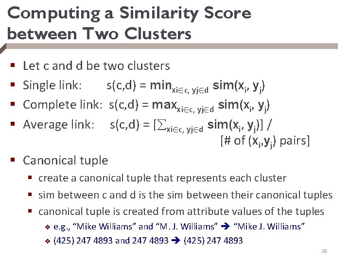
Computing a Similarity Score between Two Clusters Let c and d be two clusters Single link: s(c, d) = minxi 2 c, yj 2 d sim(xi, yj) Complete link: s(c, d) = maxxi 2 c, yj 2 d sim(xi, yj) Average link: s(c, d) = [ xi 2 c, yj 2 d sim(xi, yj)] / [# of (xi, yj) pairs] § Canonical tuple § § § create a canonical tuple that represents each cluster § sim between c and d is the sim between their canonical tuples § canonical tuple is created from attribute values of the tuples e. g. , “Mike Williams” and “M. J. Williams” “Mike J. Williams” v (425) 247 4893 and 247 4893 (425) 247 4893 v 29

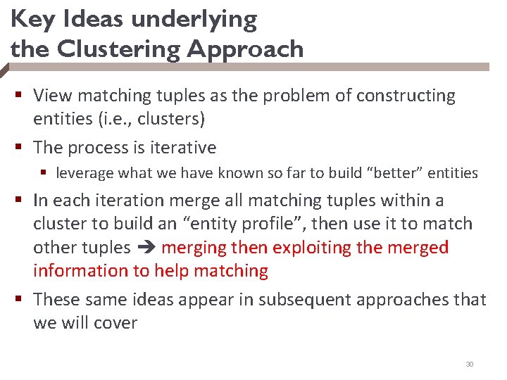
Key Ideas underlying the Clustering Approach § View matching tuples as the problem of constructing entities (i. e. , clusters) § The process is iterative § leverage what we have known so far to build “better” entities § In each iteration merge all matching tuples within a cluster to build an “entity profile”, then use it to match other tuples merging then exploiting the merged information to help matching § These same ideas appear in subsequent approaches that we will cover 30

Outline § § § Problem definition Rule-based matching Learning- based matching Matching by clustering Scaling up data matching 31

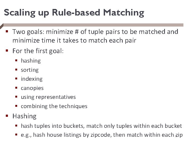
Scaling up Rule-based Matching § Two goals: minimize # of tuple pairs to be matched and minimize time it takes to match each pair § For the first goal: § § § hashing sorting indexing canopies using representatives combining the techniques § Hashing § hash tuples into buckets, match only tuples within each bucket § e. g. , hash house listings by zipcode, then match within each zip 32

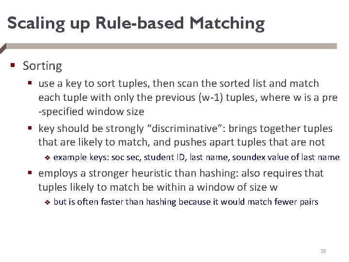
Scaling up Rule-based Matching § Sorting § use a key to sort tuples, then scan the sorted list and match each tuple with only the previous (w-1) tuples, where w is a pre -specified window size § key should be strongly “discriminative”: brings together tuples that are likely to match, and pushes apart tuples that are not v example keys: soc sec, student ID, last name, soundex value of last name § employs a stronger heuristic than hashing: also requires that tuples likely to match be within a window of size w v but is often faster than hashing because it would match fewer pairs 33

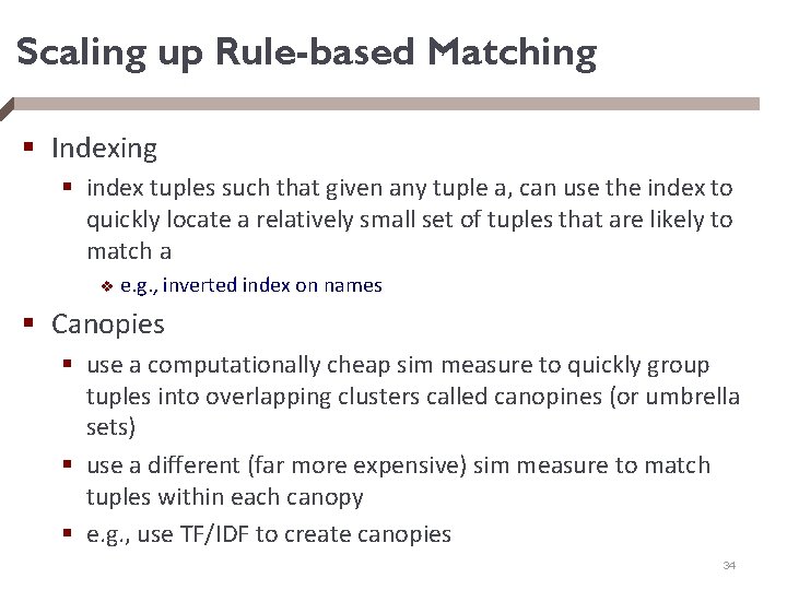
Scaling up Rule-based Matching § Indexing § index tuples such that given any tuple a, can use the index to quickly locate a relatively small set of tuples that are likely to match a v e. g. , inverted index on names § Canopies § use a computationally cheap sim measure to quickly group tuples into overlapping clusters called canopines (or umbrella sets) § use a different (far more expensive) sim measure to match tuples within each canopy § e. g. , use TF/IDF to create canopies 34

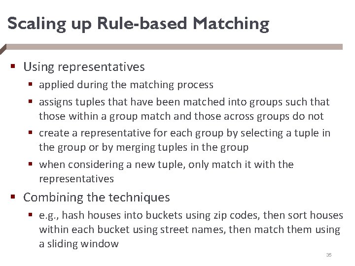
Scaling up Rule-based Matching § Using representatives § applied during the matching process § assigns tuples that have been matched into groups such that those within a group match and those across groups do not § create a representative for each group by selecting a tuple in the group or by merging tuples in the group § when considering a new tuple, only match it with the representatives § Combining the techniques § e. g. , hash houses into buckets using zip codes, then sort houses within each bucket using street names, then match them using a sliding window 35

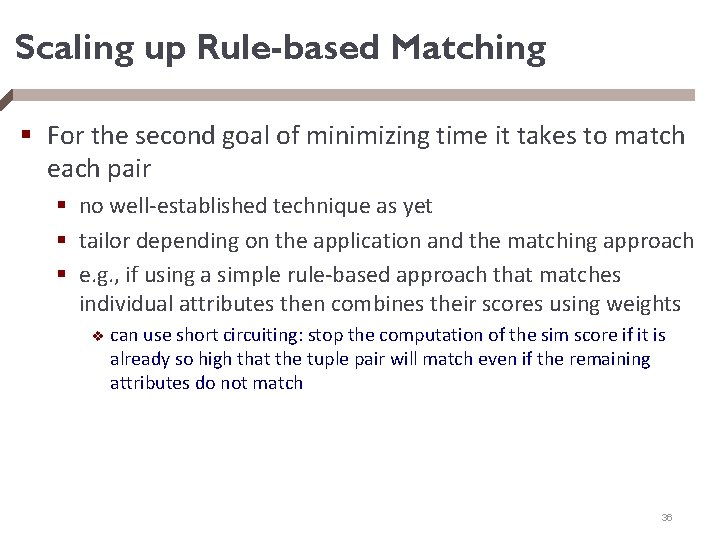
Scaling up Rule-based Matching § For the second goal of minimizing time it takes to match each pair § no well-established technique as yet § tailor depending on the application and the matching approach § e. g. , if using a simple rule-based approach that matches individual attributes then combines their scores using weights v can use short circuiting: stop the computation of the sim score if it is already so high that the tuple pair will match even if the remaining attributes do not match 36

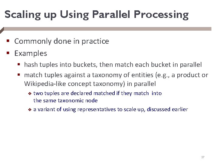
Scaling up Using Parallel Processing § Commonly done in practice § Examples § hash tuples into buckets, then match each bucket in parallel § match tuples against a taxonomy of entities (e. g. , a product or Wikipedia-like concept taxonomy) in parallel two tuples are declared matched if they match into the same taxonomic node v a variant of using representatives to scale up, discussed earlier v 37