Chapter 7 CPU Scheduling Chapter 7 CPU Scheduling

Chapter 7: CPU Scheduling

Chapter 7: CPU Scheduling n Basic Concepts n Scheduling Criteria n Scheduling Algorithms n Algorithm Evaluation Objectives n Describe various CPU scheduling algorithms n Assess CPU scheduling algorithms based on scheduling criteria n Apply modeling and simulations to evaluate CPU scheduling algorithms

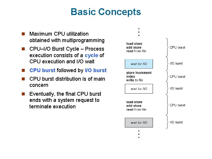
Basic Concepts n Maximum CPU utilization obtained with multiprogramming n CPU–I/O Burst Cycle – Process execution consists of a cycle of CPU execution and I/O wait n CPU burst followed by I/O burst n CPU burst distribution is of main concern n Eventually, the final CPU burst ends with a system request to terminate execution

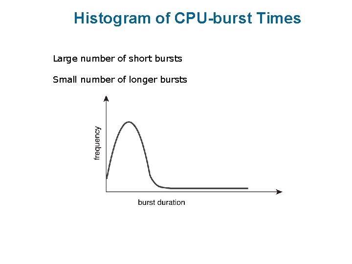
Histogram of CPU-burst Times Large number of short bursts Small number of longer bursts

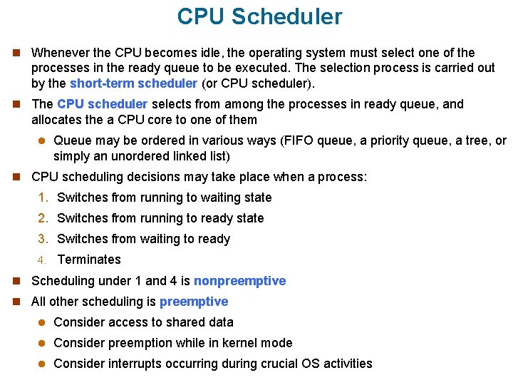
CPU Scheduler n Whenever the CPU becomes idle, the operating system must select one of the processes in the ready queue to be executed. The selection process is carried out by the short-term scheduler (or CPU scheduler). n The CPU scheduler selects from among the processes in ready queue, and allocates the a CPU core to one of them l Queue may be ordered in various ways (FIFO queue, a priority queue, a tree, or simply an unordered linked list) n CPU scheduling decisions may take place when a process: 1. Switches from running to waiting state 2. Switches from running to ready state 3. Switches from waiting to ready 4. Terminates n Scheduling under 1 and 4 is nonpreemptive n All other scheduling is preemptive l Consider access to shared data l Consider preemption while in kernel mode l Consider interrupts occurring during crucial OS activities

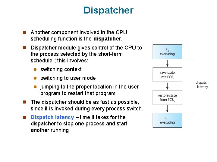
Dispatcher n Another component involved in the CPU scheduling function is the dispatcher. n Dispatcher module gives control of the CPU to the process selected by the short-term scheduler; this involves: l switching context l switching to user mode l jumping to the proper location in the user program to restart that program n The dispatcher should be as fast as possible, since it is invoked during every process switch. n Dispatch latency – time it takes for the dispatcher to stop one process and start another running

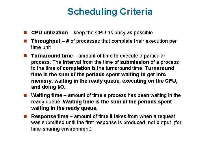
Scheduling Criteria n CPU utilization – keep the CPU as busy as possible n Throughput – # of processes that complete their execution per time unit n Turnaround time – amount of time to execute a particular process. The interval from the time of submission of a process to the time of completion is the turnaround time. Turnaround time is the sum of the periods spent waiting to get into memory, waiting in the ready queue, executing on the CPU, and doing I/O. n Waiting time – amount of time a process has been waiting in the ready queue. Waiting time is the sum of the periods spent waiting in the ready queue. n Response time – amount of time it takes from when a request was submitted until the first response is produced, not output (for time-sharing environment)

Scheduling Algorithm Optimization Criteria n Max CPU utilization n Max throughput n Min turnaround time n Min waiting time n Min response time

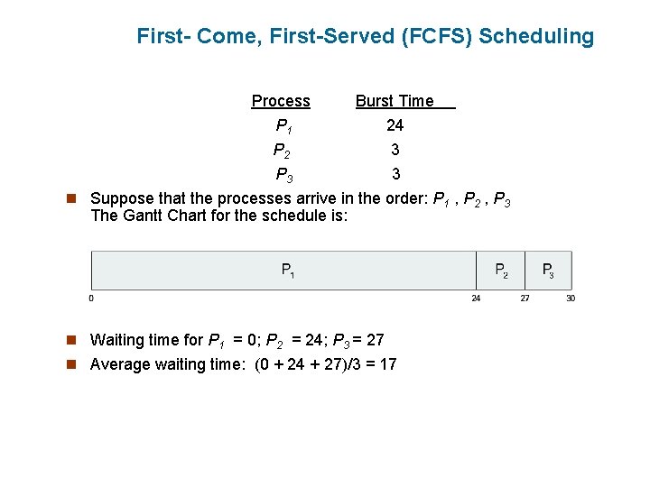
First- Come, First-Served (FCFS) Scheduling Process Burst Time P 1 24 P 2 3 P 3 3 n Suppose that the processes arrive in the order: P 1 , P 2 , P 3 The Gantt Chart for the schedule is: n Waiting time for P 1 = 0; P 2 = 24; P 3 = 27 n Average waiting time: (0 + 24 + 27)/3 = 17

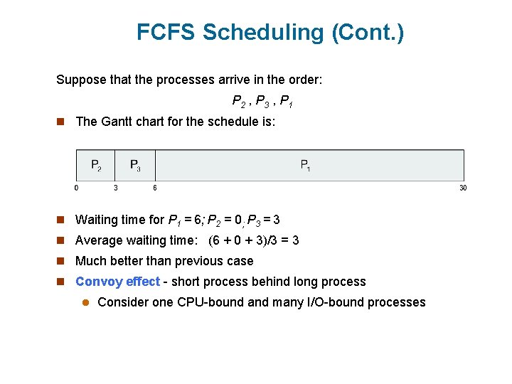
FCFS Scheduling (Cont. ) Suppose that the processes arrive in the order: P 2 , P 3 , P 1 n The Gantt chart for the schedule is: n Waiting time for P 1 = 6; P 2 = 0; P 3 = 3 n Average waiting time: (6 + 0 + 3)/3 = 3 n Much better than previous case n Convoy effect - short process behind long process l Consider one CPU-bound and many I/O-bound processes

Shortest-Job-First (SJF) Scheduling n Associate with each process the length of its next CPU burst l Use these lengths to schedule the process with the shortest time n SJF is optimal – gives minimum average waiting time for a given set of processes l The difficulty is knowing the length of the next CPU request l Could ask the user

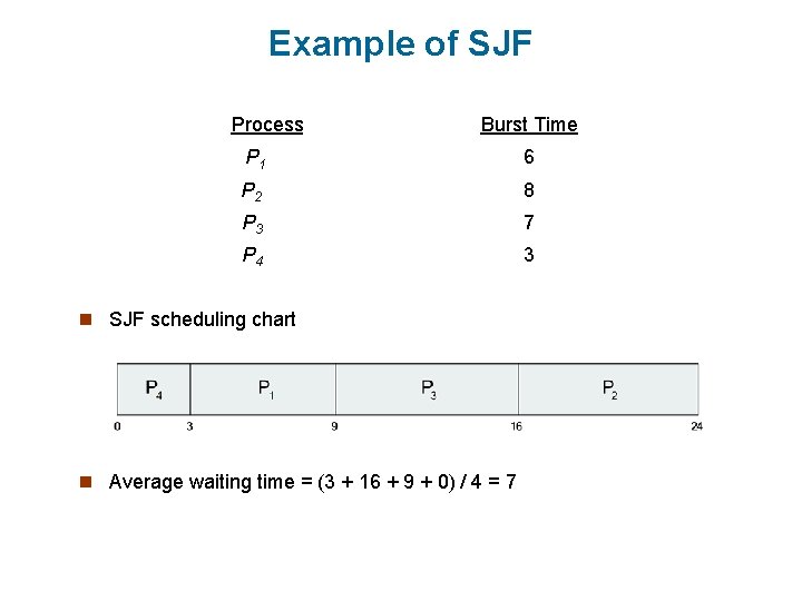
Example of SJF Process. Arrival Time Burst Time P 1 0. 0 6 P 2 2. 0 8 P 3 4. 0 7 P 4 5. 0 3 n SJF scheduling chart n Average waiting time = (3 + 16 + 9 + 0) / 4 = 7

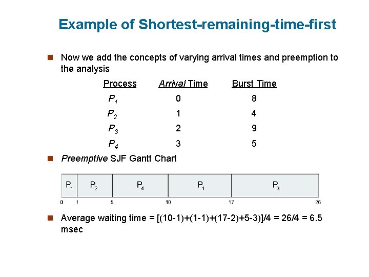
Example of Shortest-remaining-time-first n Now we add the concepts of varying arrival times and preemption to the analysis Process. Aarri Arrival Time. T Burst Time P 1 0 8 P 2 1 4 P 3 2 9 P 4 3 5 n Preemptive SJF Gantt Chart n Average waiting time = [(10 -1)+(17 -2)+5 -3)]/4 = 26/4 = 6. 5 msec

Round Robin (RR) n Each process gets a small unit of CPU time (time quantum q), usually 10 -100 milliseconds. After this time has elapsed, the process is preempted and added to the end of the ready queue. n If there are n processes in the ready queue and the time quantum is q, then each process gets 1/n of the CPU time in chunks of at most q time units at once. No process waits more than (n-1)q time units. n Timer interrupts every quantum to schedule next process n Performance l q large FIFO l q small q must be large with respect to context switch, otherwise overhead is too high

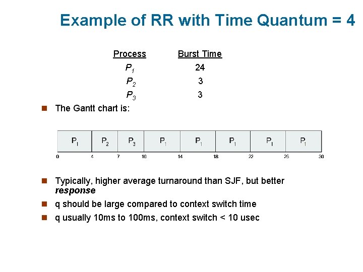
Example of RR with Time Quantum = 4 Process P 1 P 2 P 3 n The Gantt chart is: Burst Time 24 3 3 n Typically, higher average turnaround than SJF, but better response n q should be large compared to context switch time n q usually 10 ms to 100 ms, context switch < 10 usec

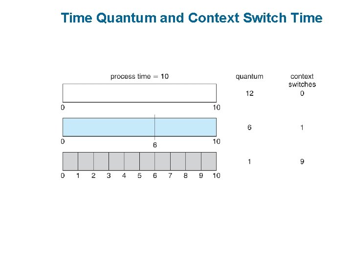
Time Quantum and Context Switch Time

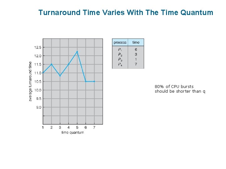
Turnaround Time Varies With The Time Quantum 80% of CPU bursts should be shorter than q

Priority Scheduling n A priority number (integer) is associated with each process n The CPU is allocated to the process with the highest priority (smallest integer highest priority) l Preemptive l Nonpreemptive n Priorities can be defined either internally or externally. 1. Internally defined priorities use some measurable quantity or quantities to compute the priority of a process. For example, time limits, memory requirements, the number of open files, and the ratio of average I/O burst to average CPU burst have been used in computing priorities. 2. Externally priorities are set by criteria that are external to the operating system, such as the importance of the process, the type and amount of funds being paid for computer use, the department sponsoring the work, and other, often political, factors. n Problem Starvation – low priority processes may never execute n Solution Aging – as time progresses increase the priority of the process

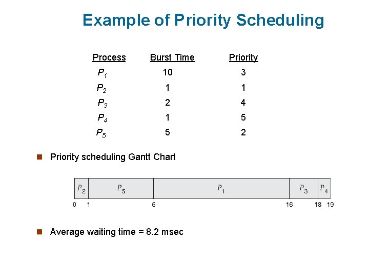
Example of Priority Scheduling Process. A arri Burst Time. T Priority P 1 10 3 P 2 1 1 P 3 2 4 P 4 1 5 P 5 5 2 n Priority scheduling Gantt Chart n Average waiting time = 8. 2 msec

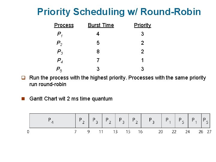
Priority Scheduling w/ Round-Robin Process. A arri Burst Time. T Priority P 1 4 3 P 2 5 2 P 3 8 2 P 4 7 1 P 5 3 3 q Run the process with the highest priority. Processes with the same priority run round-robin n Gantt Chart wit 2 ms time quantum

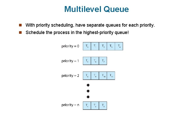
Multilevel Queue n With priority scheduling, have separate queues for each priority. n Schedule the process in the highest-priority queue!

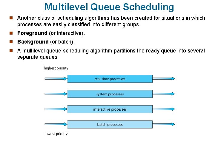
Multilevel Queue Scheduling n Another class of scheduling algorithms has been created for situations in which processes are easily classified into different groups. n Foreground (or interactive). n Background (or batch). n A multilevel queue-scheduling algorithm partitions the ready queue into several separate queues

Multilevel Queue Scheduling n The processes are permanently assigned to one queue, generally based on some property of the process, such as: 1. memory size 2. process priority, or 3. process type. Processes do not move between queues, since processes do not change their foreground or background nature. n Each queue has its own scheduling algorithm. n The foreground queue might be scheduled by an RR algorithm. n The background queue is scheduled by an FCFS algorithm

Multilevel Feedback Queue Scheduling n A process can move between the various queues; aging can be implemented this way n Multilevel-feedback-queue scheduler defined by the following parameters: l number of queues l scheduling algorithms for each queue l method used to determine when to upgrade a process l method used to determine when to demote a process l method used to determine which queue a process will enter when that process needs service

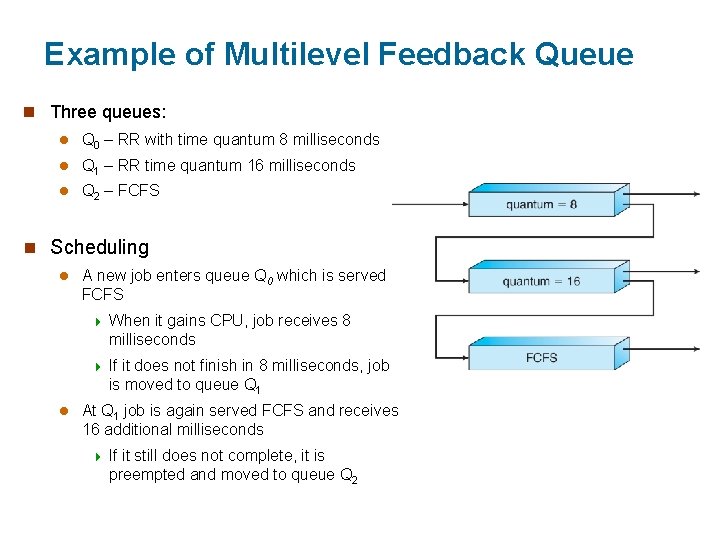
Example of Multilevel Feedback Queue n Three queues: l Q 0 – RR with time quantum 8 milliseconds l Q 1 – RR time quantum 16 milliseconds l Q 2 – FCFS n Scheduling l l A new job enters queue Q 0 which is served FCFS 4 When it gains CPU, job receives 8 milliseconds 4 If it does not finish in 8 milliseconds, job is moved to queue Q 1 At Q 1 job is again served FCFS and receives 16 additional milliseconds 4 If it still does not complete, it is preempted and moved to queue Q 2

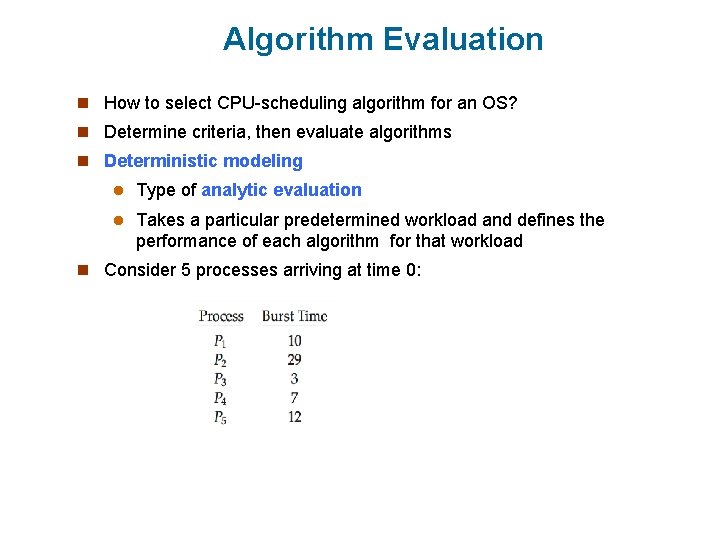
Algorithm Evaluation n How to select CPU-scheduling algorithm for an OS? n Determine criteria, then evaluate algorithms n Deterministic modeling l Type of analytic evaluation l Takes a particular predetermined workload and defines the performance of each algorithm for that workload n Consider 5 processes arriving at time 0:

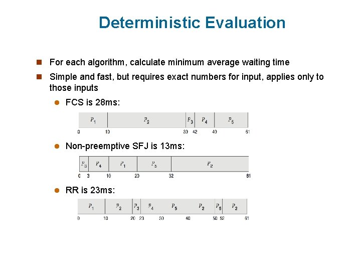
Deterministic Evaluation n For each algorithm, calculate minimum average waiting time n Simple and fast, but requires exact numbers for input, applies only to those inputs l FCS is 28 ms: l Non-preemptive SFJ is 13 ms: l RR is 23 ms:

Queueing Models n Describes the arrival of processes, and CPU and I/O bursts probabilistically l Commonly exponential, and described by mean l Computes average throughput, utilization, waiting time, etc n Computer system described as network of servers, each with queue of waiting processes l Knowing arrival rates and service rates l Computes utilization, average queue length, average wait time, etc

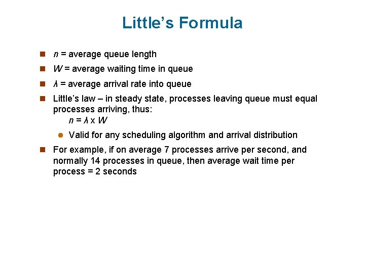
Little’s Formula n n = average queue length n W = average waiting time in queue n λ = average arrival rate into queue n Little’s law – in steady state, processes leaving queue must equal processes arriving, thus: n=λx. W l Valid for any scheduling algorithm and arrival distribution n For example, if on average 7 processes arrive per second, and normally 14 processes in queue, then average wait time per process = 2 seconds

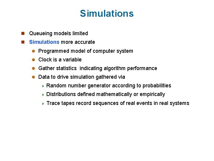
Simulations n Queueing models limited n Simulations more accurate l Programmed model of computer system l Clock is a variable l Gather statistics indicating algorithm performance l Data to drive simulation gathered via 4 Random number generator according to probabilities 4 Distributions 4 Trace defined mathematically or empirically tapes record sequences of real events in real systems

End of Chapter 7