Chapter 7 Correlation and Simple Linear Regression 1

Chapter 7: Correlation and Simple Linear Regression 1

Introduction • Often, scientists and engineers collect data in order to determine the nature of the relationship between two quantities. • An example is: heights and forearm lengths of men. • Many times, this ordered pairs of measurements, fall approximately along a straight line when plotted. • In those situations, the data can be used to compute an equation for the line that “best fits” the data. • This line can be used for various things, one is predicting for future values. 2

Section 7. 1: Correlation • Something we may be interested in is how closely related two physical characteristics are. For example, height and weight of a two year old. • The quantity called the correlation coefficient is a measure of this. • We look at the direction of the relationship, positive or negative, strength of relationship, and then we find a line that best fits the data. • In computing correlation, we can only use quantitative data. 3

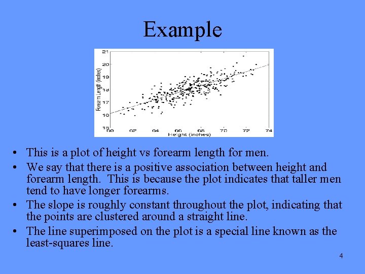
Example • This is a plot of height vs forearm length for men. • We say that there is a positive association between height and forearm length. This is because the plot indicates that taller men tend to have longer forearms. • The slope is roughly constant throughout the plot, indicating that the points are clustered around a straight line. • The line superimposed on the plot is a special line known as the least-squares line. 4

Correlation Coefficient • The degree to which the points in a scatterplot tend to cluster around a line reflects the strength of the linear relationship between x and y. • The correlation coefficient is a numerical measure of the strength of the linear relationship between two variables. • The correlation coefficient is usually denoted by the letter r. 5

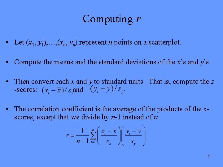
Computing r • Let (x 1, y 1), …, (xn, yn) represent n points on a scatterplot. • Compute the means and the standard deviations of the x’s and y’s. • Then convert each x and y to standard units. That is, compute the z -scores: and • The correlation coefficient is the average of the products of the zscores, except that we divide by n-1 instead of n. 6

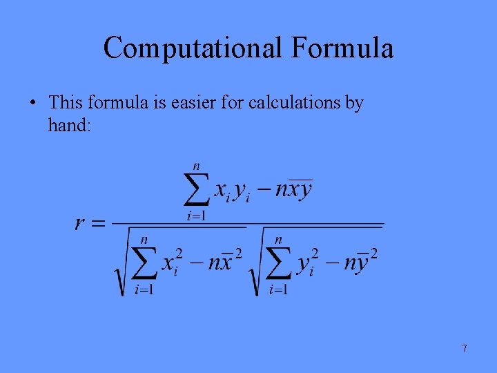
Computational Formula • This formula is easier for calculations by hand: 7

Comments • In principle, the correlation coefficient can be calculated for any set of points. • In many cases, the points constitute a random sample from a population of points. • In this case, the correlation coefficient is called the sample correlation, and it is an estimate of the population correlation. 8

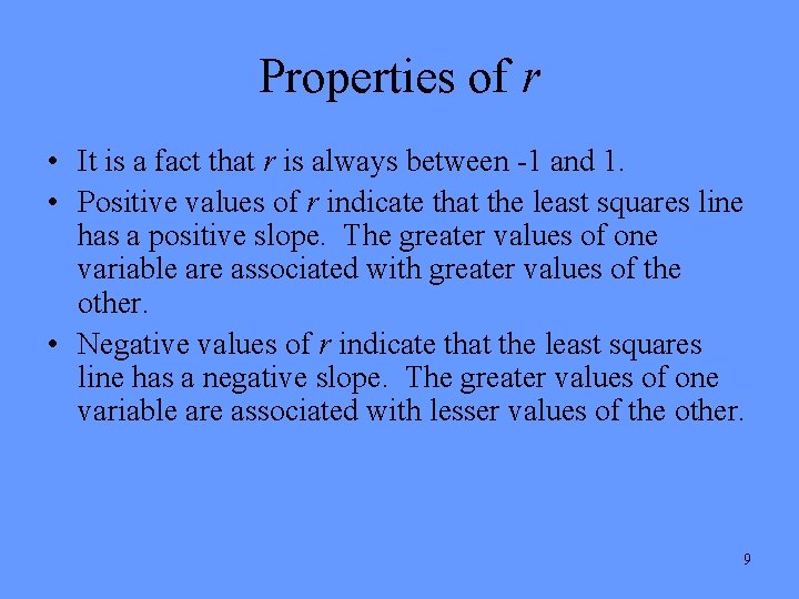
Properties of r • It is a fact that r is always between -1 and 1. • Positive values of r indicate that the least squares line has a positive slope. The greater values of one variable are associated with greater values of the other. • Negative values of r indicate that the least squares line has a negative slope. The greater values of one variable are associated with lesser values of the other. 9

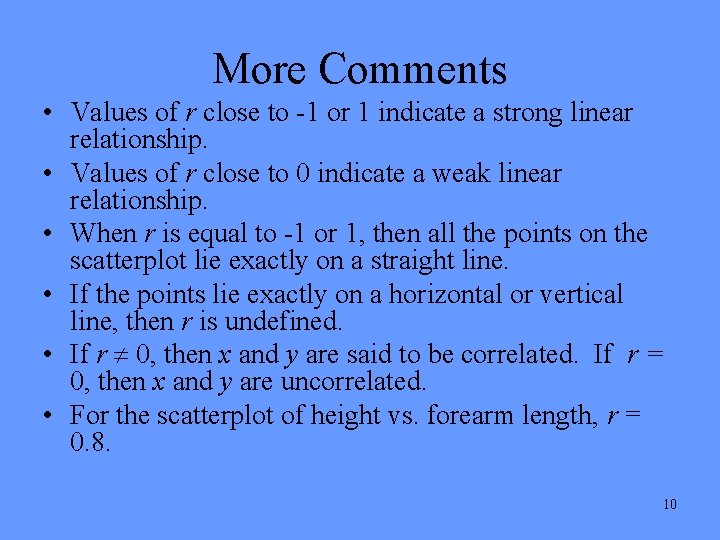
More Comments • Values of r close to -1 or 1 indicate a strong linear relationship. • Values of r close to 0 indicate a weak linear relationship. • When r is equal to -1 or 1, then all the points on the scatterplot lie exactly on a straight line. • If the points lie exactly on a horizontal or vertical line, then r is undefined. • If r 0, then x and y are said to be correlated. If r = 0, then x and y are uncorrelated. • For the scatterplot of height vs. forearm length, r = 0. 8. 10

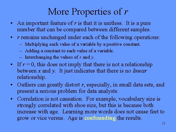
More Properties of r • An important feature of r is that it is unitless. It is a pure number that can be compared between different samples. • r remains unchanged under each of the following operations: – Multiplying each value of a variable by a positive constant. – Adding a constant to each value of a variable. – Interchanging the values of x and y. • If r = 0, this does not imply that there is not a relationship between x and y. It just indicates that there is no linear relationship. • Outliers can greatly distort r, especially, in small data sets, and present a serious problem for data analysts. • Correlation is not causation. For example, vocabulary size is strongly correlated with shoe size, but this is because both increase with age. Learning more words does not cause feet to grow or vice versus. Age is confounding the results. 11

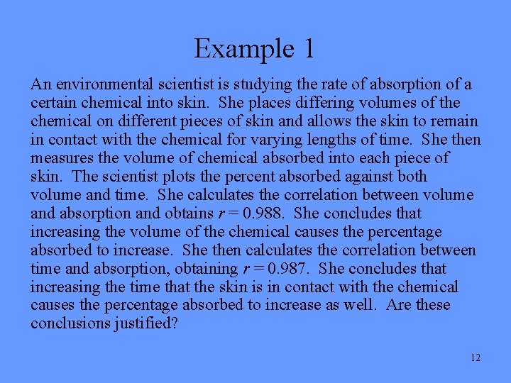
Example 1 An environmental scientist is studying the rate of absorption of a certain chemical into skin. She places differing volumes of the chemical on different pieces of skin and allows the skin to remain in contact with the chemical for varying lengths of time. She then measures the volume of chemical absorbed into each piece of skin. The scientist plots the percent absorbed against both volume and time. She calculates the correlation between volume and absorption and obtains r = 0. 988. She concludes that increasing the volume of the chemical causes the percentage absorbed to increase. She then calculates the correlation between time and absorption, obtaining r = 0. 987. She concludes that increasing the time that the skin is in contact with the chemical causes the percentage absorbed to increase as well. Are these conclusions justified? 12

Inference on the Population Correlation If the random variables X and Y have a certain joint distribution called a bivariate normal distribution, then the sample correlation r can be used to construct confidence intervals and perform hypothesis tests on the population correlation, ρ. The following results make this possible. 13

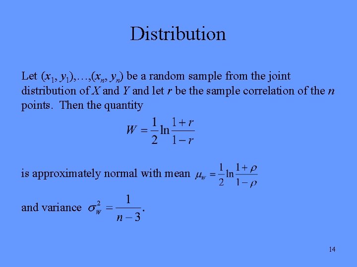
Distribution Let (x 1, y 1), …, (xn, yn) be a random sample from the joint distribution of X and Y and let r be the sample correlation of the n points. Then the quantity is approximately normal with mean and variance 14

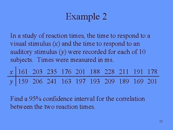
Example 2 In a study of reaction times, the time to respond to a visual stimulus (x) and the time to respond to an auditory stimulus (y) were recorded for each of 10 subjects. Times were measured in ms. x 161 203 235 176 201 188 228 211 191 178 y 159 206 241 163 197 193 209 189 169 201 Find a 95% confidence interval for the correlation between the two reaction times. 15

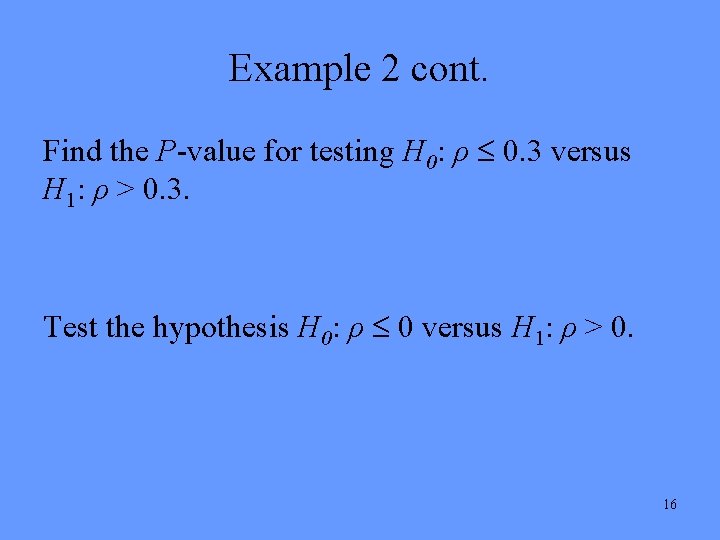
Example 2 cont. Find the P-value for testing H 0: ρ 0. 3 versus H 1: ρ > 0. 3. Test the hypothesis H 0: ρ 0 versus H 1: ρ > 0. 16

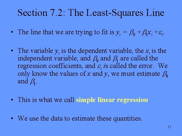
Section 7. 2: The Least-Squares Line • The line that we are trying to fit is yi = 0 + 1 xi + i. • The variable yi is the dependent variable, the xi is the independent variable, and 0 and 1 are called the regression coefficients, and i is called the error. We only know the values of x and y, we must estimate 0 and 1. • This is what we call simple linear regression. • We use the data to estimate these quantities. 17

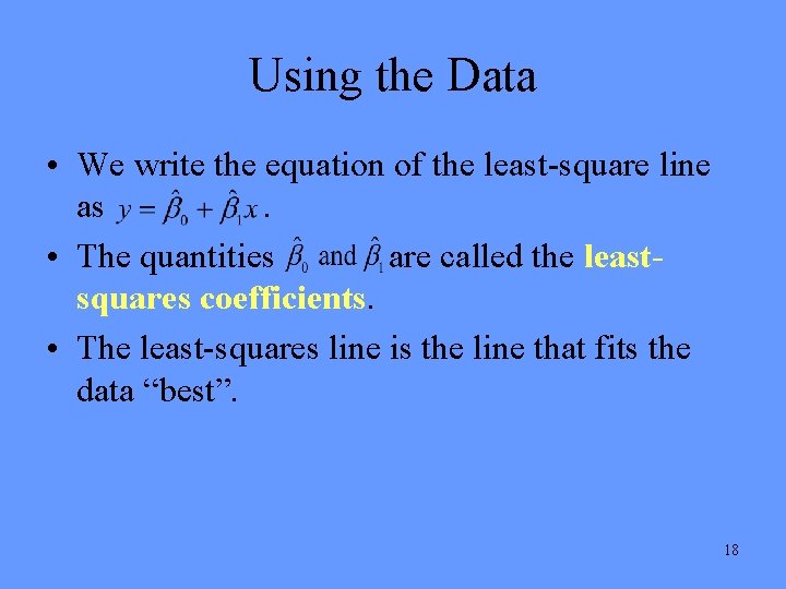
Using the Data • We write the equation of the least-square line as. • The quantities are called the leastsquares coefficients. • The least-squares line is the line that fits the data “best”. 18

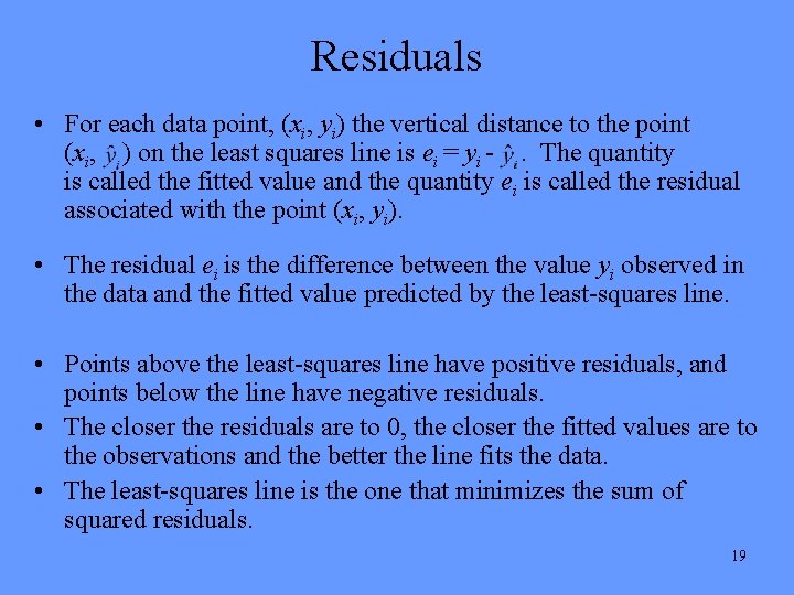
Residuals • For each data point, (xi, yi) the vertical distance to the point (xi, ) on the least squares line is ei = yi -. The quantity is called the fitted value and the quantity ei is called the residual associated with the point (xi, yi). • The residual ei is the difference between the value yi observed in the data and the fitted value predicted by the least-squares line. • Points above the least-squares line have positive residuals, and points below the line have negative residuals. • The closer the residuals are to 0, the closer the fitted values are to the observations and the better the line fits the data. • The least-squares line is the one that minimizes the sum of squared residuals. 19

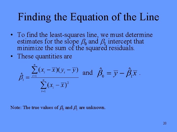
Finding the Equation of the Line • To find the least-squares line, we must determine estimates for the slope 0 and 1 intercept that minimize the sum of the squared residuals. • These quantities are and . Note: The true values of 0 and 1 are unknown. 20

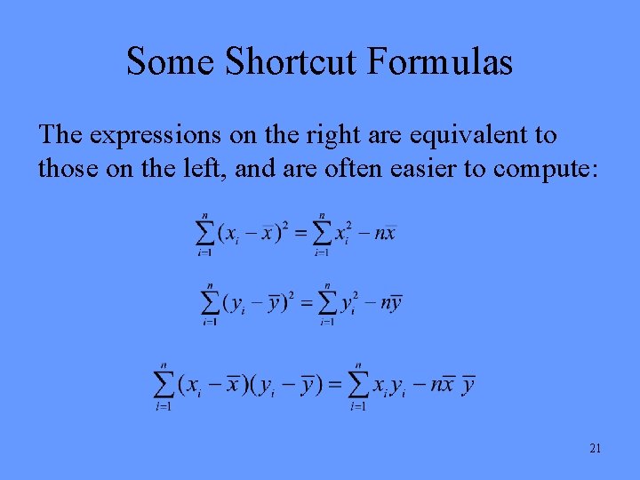
Some Shortcut Formulas The expressions on the right are equivalent to those on the left, and are often easier to compute: 21

Example 2 cont. Using the data in Example 2, compute the least-squares estimates of the spring constant and the unloaded length of the spring. Write the equation of the least-sqaures line. Estimate the time to respond if the visual stimulus time is 200. 22

Cautions • Do not extrapolate the fitted line (such as the leastsquares line) outside the range of the data. The linear relationship may not hold there. • We learned that we should not use the correlation coefficient when the relationship between x and y is not linear. The same holds for the least-squares line. When the scatterplot follows a curved pattern, it does not make sense to summarize it with a straight line. • If the relationship is curved, then we would want to fit a regression line that contain squared terms. 23

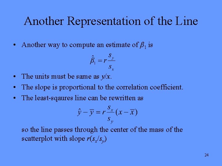
Another Representation of the Line • Another way to compute an estimate of β 1 is • The units must be same as y/x. • The slope is proportional to the correlation coefficient. • The least-sqaures line can be rewritten as so the line passes through the center of the mass of the scatterplot with slope r(sx/sy) 24

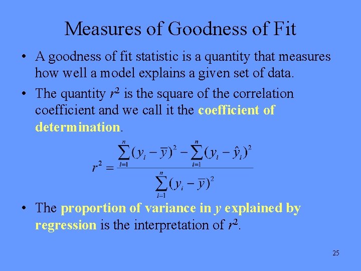
Measures of Goodness of Fit • A goodness of fit statistic is a quantity that measures how well a model explains a given set of data. • The quantity r 2 is the square of the correlation coefficient and we call it the coefficient of determination. • The proportion of variance in y explained by regression is the interpretation of r 2. 25

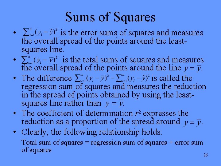
Sums of Squares • • • is the error sums of squares and measures the overall spread of the points around the leastsquares line. is the total sums of squares and measures the overall spread of the points around the line. The difference is called the regression sum of squares and measures the reduction in the spread of points obtained by using the leastsquares line rather than. The coefficient of determination r 2 expresses the reduction as a proportion of the spread around. Clearly, the following relationship holds: Total sum of squares = regression sum of squares + error sum of squares 26

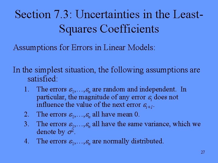
Section 7. 3: Uncertainties in the Least. Squares Coefficients Assumptions for Errors in Linear Models: In the simplest situation, the following assumptions are satisfied: 1. The errors 1, …, n are random and independent. In particular, the magnitude of any error i does not influence the value of the next error i+1. 2. The errors 1, …, n all have mean 0. 3. The errors 1, …, n all have the same variance, which we denote by 2. 4. The errors 1, …, n are normally distributed. 27

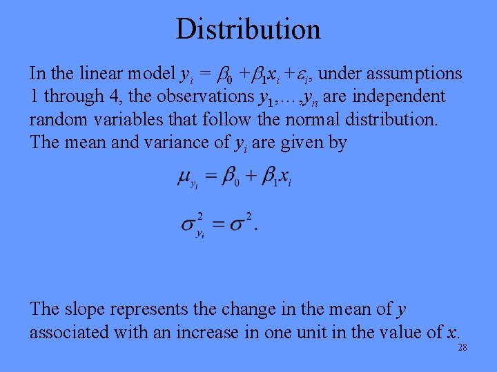
Distribution In the linear model yi = 0 + 1 xi + i, under assumptions 1 through 4, the observations y 1, …, yn are independent random variables that follow the normal distribution. The mean and variance of yi are given by The slope represents the change in the mean of y associated with an increase in one unit in the value of x. 28

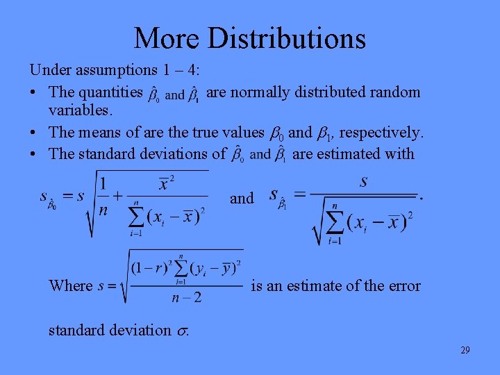
More Distributions Under assumptions 1 – 4: • The quantities are normally distributed random variables. • The means of are the true values 0 and 1, respectively. • The standard deviations of are estimated with and Where is an estimate of the error standard deviation . 29

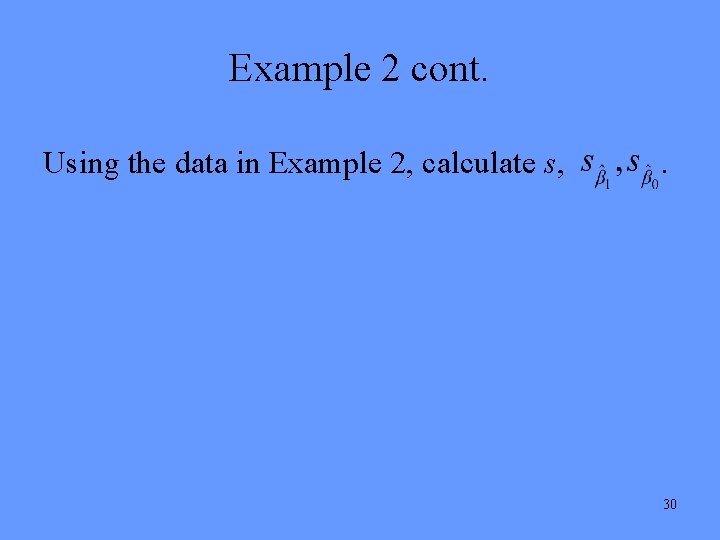
Example 2 cont. Using the data in Example 2, calculate s, . 30

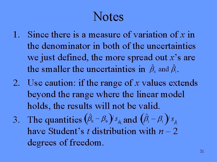
Notes 1. Since there is a measure of variation of x in the denominator in both of the uncertainties we just defined, the more spread out x’s are the smaller the uncertainties in. 2. Use caution: if the range of x values extends beyond the range where the linear model holds, the results will not be valid. 3. The quantities and have Student’s t distribution with n – 2 degrees of freedom. 31

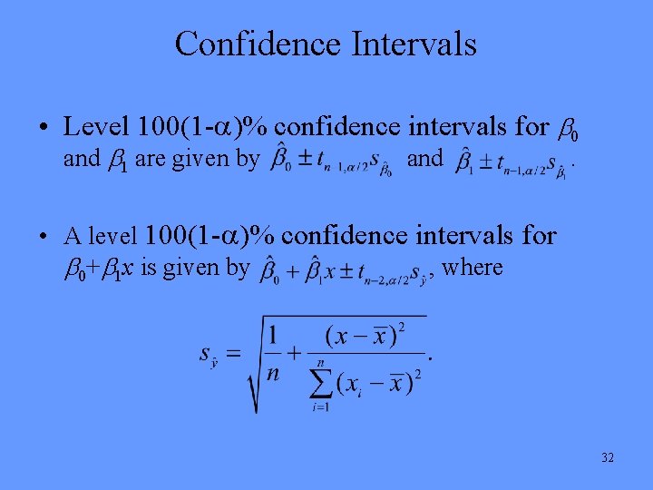
Confidence Intervals • Level 100(1 - )% confidence intervals for 0 and 1 are given by and . • A level 100(1 - )% confidence intervals for 0+ 1 x is given by , where 32

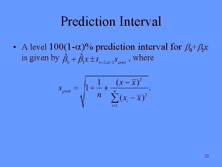
Prediction Interval • A level 100(1 - )% prediction interval for 0+ 1 x is given by , where 33

Example 2 cont. For the data in Example 2, compute a confidence interval for the slope of the regression line. 34

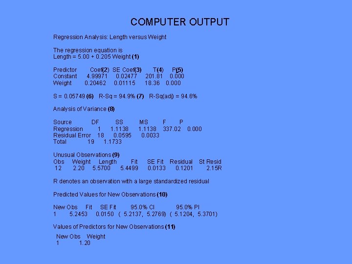
COMPUTER OUTPUT Regression Analysis: Length versus Weight The regression equation is Length = 5. 00 + 0. 205 Weight (1) Predictor Constant Weight Coef(2) SE Coef(3) T(4) P(5) 4. 99971 0. 02477 201. 81 0. 000 0. 20462 0. 01115 18. 36 0. 000 S = 0. 05749 (6) R-Sq = 94. 9% (7) R-Sq(adj) = 94. 6% Analysis of Variance (8) Source DF SS Regression 1 1. 1138 Residual Error 18 0. 0595 Total 19 1. 1733 Unusual Observations (9) Obs Weight Length Fit 12 2. 20 5. 5700 5. 4499 MS F P 1. 1138 337. 02 0. 000 0. 0033 SE Fit Residual St Resid 0. 0133 0. 1201 2. 15 R R denotes an observation with a large standardized residual Predicted Values for New Observations (10) New Obs Fit SE Fit 95. 0% CI 95. 0% PI 1 5. 2453 0. 0150 ( 5. 2137, 5. 2769) ( 5. 1204, 5. 3701) Values of Predictors for New Observations (11) New Obs Weight 1 1. 20

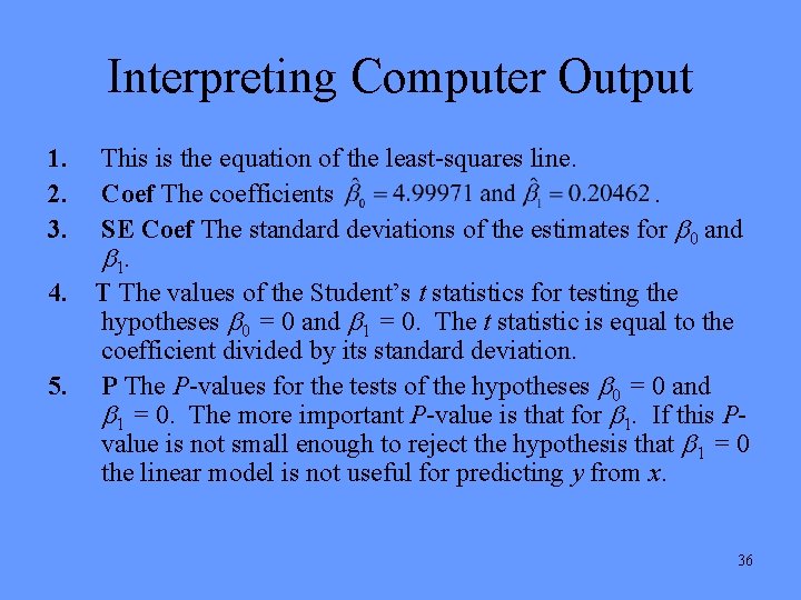
Interpreting Computer Output 1. 2. 3. 4. 5. This is the equation of the least-squares line. Coef The coefficients. SE Coef The standard deviations of the estimates for 0 and 1. T The values of the Student’s t statistics for testing the hypotheses 0 = 0 and 1 = 0. The t statistic is equal to the coefficient divided by its standard deviation. P The P-values for the tests of the hypotheses 0 = 0 and 1 = 0. The more important P-value is that for 1. If this Pvalue is not small enough to reject the hypothesis that 1 = 0 the linear model is not useful for predicting y from x. 36

More Computer Output Interpretation 6. 7. S The estimate of s, the error standard deviation. R-Sq This is r 2, the square of the correlation coefficient r, also called the coefficient of determination. 8. Analysis of Variance This table is not so important in simple linear regression, we will discuss it when we discuss multiple linear regression. 9. Unusual Observations Minitab tries to alert you to data points that may violate the assumptions 1 -4. 10. Predicted Values for New Observations These are confidence intervals and prediction intervals for values of x specified by the user. 11. Values of Predictors for New Observations This is simply a list of the x values for which confidence and prediction intervals have been calculated. 37

Section 7. 4: Checking Assumptions and Transforming Data • We stated some assumptions for the errors. Here we want to see if any of those assumptions are violated. • The single best diagnostic for least-squares regression is a plot of residuals versus the fitted values, sometimes called a residual plot. 38

More of the Residual Plot • When the linear model is valid, and assumptions 1 – 4 are satisfied, the plot will show no substantial pattern. There should be no curve to the plot, and the vertical spread of the points should not vary too much over the horizontal range of the data. • A good-looking residual plot does not by itself prove that the linear model is appropriate. However, a residual plot with a serious defect does clearly indicate that the linear model is inappropriate. 39

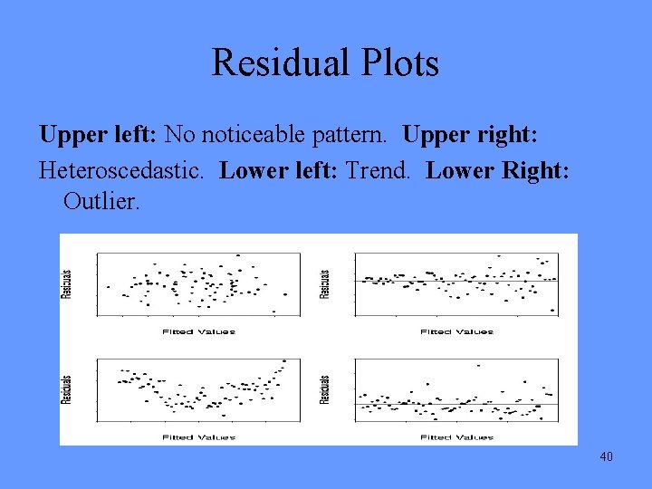
Residual Plots Upper left: No noticeable pattern. Upper right: Heteroscedastic. Lower left: Trend. Lower Right: Outlier. 40

Residuals versus Fitted Values If the plot of residuals versus fitted values • Shows no substantial trend or curve, and • Is homoscedastic, that is, the vertical spread does not vary too much along the horizontal length of plot, except perhaps near the edges. then it is likely, but not certain, that the assumptions of the linear model hold. However, if the residual plot does show a substantial trend or curve, or is heteroscedastic, it is certain that the assumptions of the linear model do not hold. 41

Transformations • If we fit the linear model y = 0 + 1 x + and find that the residual plot exhibits a trend or pattern, we can sometimes fix the problem by raising x, y, or both to a power. • It may be the case that a model of the form ya = 0 + 1 xb + fits the data well. • Replacing a variable with a function of itself is called transforming the variable. Specifically, raising a variable to a power is called a power transformation. 42

Don’t Forget • Once the transformation has been completed, then you must inspect the residual plot again to see if that model is a good fit. • It is fine to proceed through transformations by trial and error. • It is important to remember that power transformations don’t always work. 43

Caution • When there are only a few points in a residual plot, it can be hard to determine whether the assumptions of the linear model is met. • When one is faced with a sparse residual plot that is hard to interpret, a reasonable thing to do is to fit a linear model, but to consider the results tentative, with the understanding that the appropriateness of the model has not been established. 44

Outliers • Outliers are points that are detached from the bulk of the data. • Both the scatter plot and the residual plot should be examined for outliers. • The first thing to do with an outlier is to determine why it is different from the rest of the points. • Sometimes outliers are caused by data-recording errors or equipment malfunction. In this case, the outlier can be deleted from the data set. In this case, you may present results that do not include the outlier. • If it cannot be determined why there is an outlier, then it is not wise to delete it. Here the results presented, should be the ones from analysis with the outlier included in the data set. 45

Influential Point • If there are outliers that cannot be removed from the data set, then the best thing to do is fit the whole data set and then remove the outlier and fit a line to the data set. • If none of the outliers upon removal make a noticeable difference to the least-squares line or to the estimated standard deviation of the slope and intercept, then use the fit with the outliers included. • If one or more outlier does make a difference, then the range of values for the least-squares coefficients should be reported. Avoid computing confidence and prediction intervals and performing hypothesis tests. • An outlier that makes a considerable difference to the leastsquares line when removed is called an influential point. • In general, outliers with unusual x values are more likely to be influential than those with unusual y values, but every outlier should be checked. • Some authors restrict the definition of outliers to points that 46 have unusually large residuals.

Comments • Transforming the variables is not the only method for analyzing data when the residual plot indicates a problem. • There is a technique called weighted least squares regression. The effect is to make the points whose error variance is smaller have greater influence in the computation of the least-squares line. • When the residual plot shows a trend, this sometimes indicates that more than one independent variable is needed to explain the variation in the dependent variable. • If the relationship is nonlinear, then a method called nonlinear regression can be applied. • If the plot of residuals versus fitted values looks good, it may be advisable to perform additional diagnostics to further check the fit of the linear model. A time series plot is used to see if time should be included in the model. A normal probability plot can be used to check the normality assumption. 47

Independence of Observations • If the plot of residuals versus fitted values looks good, then further diagnostics may be used to further check the fit of the linear model. • A time order plot of the residuals versus order in which observations were made. • If there are trends in this plot, then x and y may be varying with time. In this case, adding a time term to the model as an additional independent variable. 48

Normality Assumption • To check that the errors are normally distributed, a normal probability plot of the residuals can be made. • If the plot looks like it follows a rough straight line, then we can conclude that the residuals are approximately normally distributed. 49

Comments • Physical laws are applicable to all future observations. • An empirical model is valid only for the data to which it is fit. It may or may not be useful in predicting outcomes for subsequent observations. • Determining whether to apply an empirical model to a future observation requires scientific judgment rather that statistical analysis. 50

Summary We discussed Ø correlation Ø least-squares line / regression Ø uncertainties in the least-squares coefficients Ø confidence intervals and hypothesis tests for leastsquares coefficients Ø checking assumptions Øresiduals 51