Chapter 7 Alternative Modeling of Binary Response Data

Chapter 7 Alternative Modeling of Binary Response Data 1

Section Review 7. 1 ---Probit and Complementary Log-Log Models 7. 2 ---Bayesian inference for binary regression 7. 3 ---Conditional Logistic regression 7. 4 ---Smoothing: Kernels, Penalized Likelihood, Generalized additive models 7. 5 ---Issues in analyzing high-dimensional categorical data 2

Review 3

Components of Generalized Linear Models 4

The link function that transforms the mean to the natural parameter is called the canonical link 5

Logit Models for Binary Data 6

7. 1 Probit and Complementary Log-Log Models 7

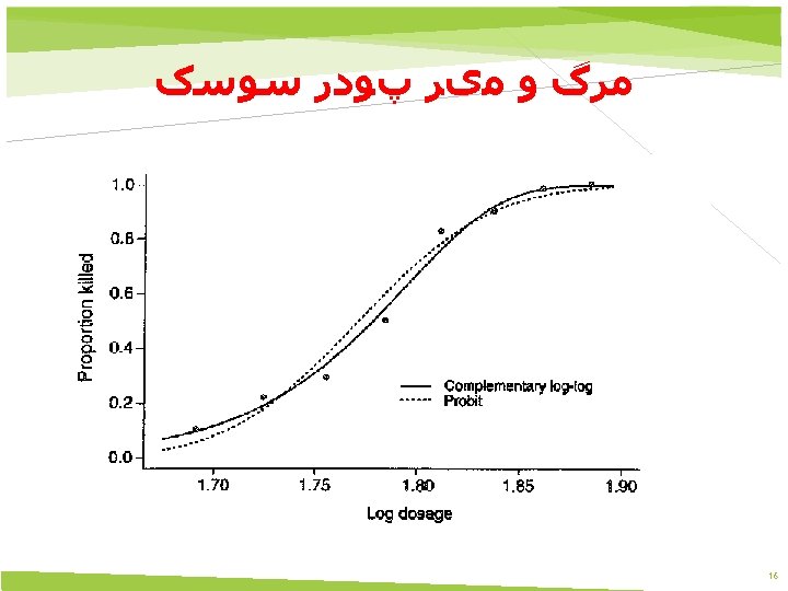
cumulative distribution function A monotone regression curve has the shape of a cumulative distribution function (cdf) for a continuous random variable. This suggests a model for a binary response having form π (x) =F( x) for some cdf F Using an entire class of locationscale cdf ’s, such as normal cdf ’s with their variety of means and variances 8

Latent Tolerance Motivation for Binary Response Models 9

Latent Tolerance Motivation for Binary Response Models 10

Probit Models 11

Tree Latent Variable Motivation Latent Tolerance Motivation for Binary Response Models Threshold Models Choice between two option, such as two product 12

Interpreting Effects 13

Probit Model Fitting 14

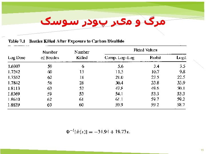
SPSS x 1. 6907 1. 7242 1. 7552 1. 7842 1. 8113 1. 8369 1. 861 1. 8839 y 6 13 18 28 52 53 61 60 n 59 60 62 56 63 59 62 60 DATASET ACTIVATE Data. Set 0. PROBIT VAR 00002 OF VAR 00003 WITH VAR 00001 /LOG NONE /MODEL PROBIT /PRINT FREQ CI /CRITERIA P(0. 15) ITERATE(20) STEPLIMIT(. 1). 17

SPSS 2 18

Complementary Log-Log Models 19

Complementary Log-Log Models 20

Extreme value 21

Complementary Log-Log Models 22

7. 2 Bayesian inference for binary regression 24

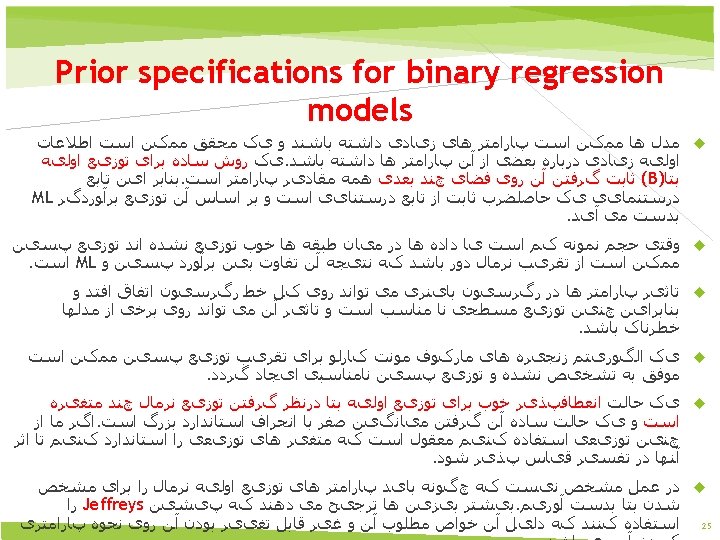
Jeffreys Priors 26

Jeffreys Priors is proper with Logit Link Probit Link Complementary Log-Log Link 27

Ex 7. 2. 2: endometrial cancer 28

Ex 7. 2. 2: endometrial cancer 29

Bayesian logistic regression for retrospective studies 30

data augmentation prior ﺗﻘﻮیﺖ ﺩﺍﺩﻩ ﻫﺎی ﺍﻭﻟیﻪ By analyzing the data using the values of mean, standard deviation, range, or clustering algorithms, it is possible for an expert to find values that are unexpected and thus erroneous. Although the correction of such data is difficult since the true value is not known, it can be resolved by setting the values to an average or other statistical value. Statistical methods can also be used to handle missing values which can be replaced by one or more plausible values, which are usually obtained by extensive data augmentation algorithms 31

Ex 7. 2. 5: Modeling the probability a Trauma patient survives 32

Ex 7. 2. 5: Modeling the probability a Trauma patient survives 33

Bayes factor 34

Bayes factor 35

Bayesian fitting for probit models Normal Priors Simple analysis is possible in the probit case using Gibbs sampling based on the normal threshold latent variable model (Albert and Chib 1993) 36

Bayesian fitting for probit models 37

Likelihood function 38

Bayesian model checking for binary regrassion Sensitivity analyses Case deletion Bayes factors AIC (deviance information criterion) Mean posterior deviance 39

7. 3 Conditional Logistic regression 40

Conditional Logistic regression ML estimators of logistic model parameters work best when the sample size n is large compared to the number of parameters. When n is small or when the number of parameters grows as n does, improved inference results using conditional maximum likelihood. The conditional likelihood refers to a conditional distribution defined for potential samples that provide the same information about the nuisance parameters that occurs in the observed sample. 41

Conditional Likelihood For subject I Let yi denote the binary response Let xij be the value of predictor j, j=1, . . . , p. The model is: substituting yi=1 gives the usual expression, such as(5. 16). Here, we explicitly separate the intercept from the coefficients of the p predictors. For N independent observations 42

Conditional Likelihood Since the sufficient statistic for α is , we condition on . Suppose that. Denote the conditional reference set of samples having the same value of as observed by 43

Small-Sample Conditional Inference for Logistic Regression As an alternative to large-sample methods, we can use the Conditional distribution to perform “exact” inference. For small samples, inference for a parameter uses the conditional distribution after eliminating all other parameters. With it, one can calculate probabilities such as P-values exactly rather than with crude approximations. Small-Sample Conditional Inference for 2× 2 Contingency Tables Small-Sample Conditional Inference for Linear Logit Model The resulting exact conditional test that β=0 is Fisher’s exact test for 2 × 2 tables Cochran-Armitage test Small-Sample Tests of Conditional Independence in 2 × K Tables the Cochran-Mantel-Haenszel test 44

Ex 7. 3. 6)Promotion Discrimination 45

Ex 7. 3. 6)Promotion Discrimination 46

7. 4 Smoothing: Kernels, Penalized Likelihood, Generalized additive models 47

How much Smoothing? 48

Smoothing Kernel Smoothing Nearest neighbors Smoothing Penalized Likelihood Firth‘s Penalized Likelihood for logistic regression 49

Kernel Smoothing Kernel estimation is a smoothing method that estimates a probability density or mass function without assuming a parametric distribution. Let K denote a matrix containing nonnegative elements and having column sums equal to 1. Kernel estimates of cell probabilities in a contingency table have form 50

Exp: 7. 4. 3 51

Exp: 7. 4. 3 52

Nearest neighbors Smoothing 53

Penalized Likelihood 54

Firth‘s Penalized Likelihood for logistic regression 55

generalized additive model (GAM) In statistics, a generalized additive model (GAM) is a generalized linear model in which the linear predictor depends linearly on unknown smooth functions of some predictor variables, and interest focuses on inference about these smooth functions. The model relates a univariate response variable, Y, to some predictor variables, xi. An exponential family distribution is specified for Y (for example normal, binomial or Poisson distributions) along with a link function g (for example the identity or log functions) relating the expected value of Y to the predictor variables via a structure such as GLM Structure GLMs Structure 56

Advantages/Disadvantages of Various Smoothing methods 57

Issues in analyzing high-dimensional categorical data Issues in selecting explanatory variables Adjusting for multiplicity The Bonferroni method The false discovery rate Other variable selection method for high-dimensional data Principle component regression 58

Gibbs Sampling 60

Gibbs sampling is named after the physicist Josiah Willard Gibbs, in reference to an analogy between the sampling algorithm and statistical physics. Gibbs sampling or a Gibbs sampler is a Markov chain Monte Carlo (MCMC) algorithm for obtaining a sequence of observations which are approximated from a specified multivariate probability distribution (i. e. from the joint probability distribution of two or more random variables), when direct sampling is difficult. In its basic version, Gibbs sampling is a special case of the Metropolis–Hastings algorithm 61

Gibbs Sampler 62

Gibbs Sampler 63

Gibbs Sampler 64

Gibbs Sampler 65