Chapter 7 Aggregate Demand Aggregate Supply Aggregate Demand

Chapter 7 Aggregate Demand Aggregate Supply

Aggregate Demand Aggregate Supply • • • Potential output is the level of output an economy can achieve when labor is employed at its natural level. Aggregate demand is the relationship between the total quantity of goods and services demanded (from all the four sources of demand) and the price level, all other determinants of spending unchanged. The aggregate demand curve is a graphical representation of aggregate demand.

1. AGGREGATE DEMAND Learning Objectives 1. Define potential output, also called the natural level of GDP. 2. Define aggregate demand, represent it using a hypothetical aggregate demand curve, and identify and explain the three effects that cause this curve to slope downward. 3. Distinguish between a change in the aggregate quantity of goods and services demanded and a change in aggregate demand. 4. Use examples to explain how each component of aggregate demand can be a possible aggregate demand shifter. 5. Explain what a multiplier is and tell how to calculate it.

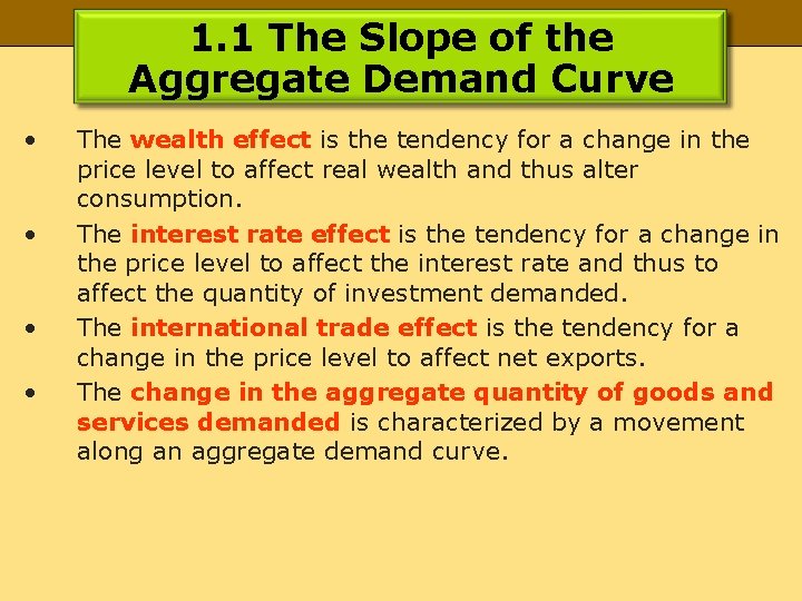
1. 1 The Slope of the Aggregate Demand Curve • • The wealth effect is the tendency for a change in the price level to affect real wealth and thus alter consumption. The interest rate effect is the tendency for a change in the price level to affect the interest rate and thus to affect the quantity of investment demanded. The international trade effect is the tendency for a change in the price level to affect net exports. The change in the aggregate quantity of goods and services demanded is characterized by a movement along an aggregate demand curve.

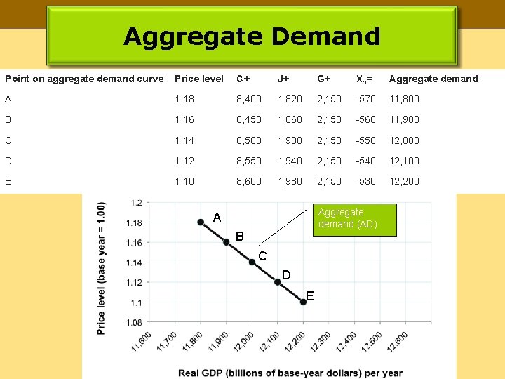
Aggregate Demand Point on aggregate demand curve Price level C+ J+ G+ Xn= Aggregate demand A 1. 18 8, 400 1, 820 2, 150 -570 11, 800 B 1. 16 8, 450 1, 860 2, 150 -560 11, 900 C 1. 14 8, 500 1, 900 2, 150 -550 12, 000 D 1. 12 8, 550 1, 940 2, 150 -540 12, 100 E 1. 10 8, 600 1, 980 2, 150 -530 12, 200 Aggregate demand (AD) A B C D E

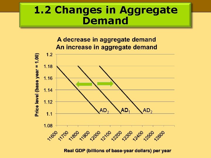
1. 2 Changes in Aggregate Demand • A Change in aggregate demand is a change in the aggregate quantity of goods and services demanded at every price level. This can be caused by changes in… – – Consumption, Investment, Government purchases, Net exports. • The exchange rate is the price of a currency in terms of another currency or currencies.

1. 2 Changes in Aggregate Demand AD 2 AD 1 AD 2

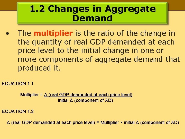
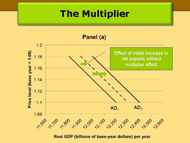
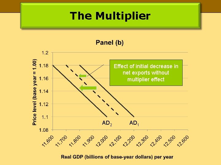
1. 2 Changes in Aggregate Demand • The multiplier is the ratio of the change in the quantity of real GDP demanded at each price level to the initial change in one or more components of aggregate demand that produced it. EQUATION 1. 1 Multiplier = Δ (real GDP demanded at each price level) initial Δ (component of AD) EQUATION 1. 2 Δ (real GDP demanded at each price level) = Multiplier × initial Δ (component of AD)

The Multiplier Effect of initial increase in net exports without multiplier effect AD 1 AD 2

The Multiplier Effect of initial decrease in net exports without multiplier effect AD 2 AD 1

2. AGGREGATE DEMAND AGGREGATE SUPPLY: THE LONG RUN AND THE SHORT RUN Learning Objectives 1. Distinguish between the short run and the long run, as these terms are used in macroeconomics. 2. Draw a hypothetical long-run aggregate supply curve and explain what it shows about the natural levels of employment and output at various price levels, given change in aggregate demand. 3. Draw a hypothetical short-run aggregate supply curve, explain why it slopes upward, and explain why it may shift; that is, distinguish between a change in the aggregate quantity of goods and services supplied and a change in short -run aggregate supply. 4. Discuss various explanations for wage and price stickiness. 5. Explain and illustrate what is meant by equilibrium in the short run and relate the equilibrium to potential output.

2. AGGREGATE DEMAND AGGREGATE SUPPLY: THE LONG RUN AND THE SHORT RUN • • • The short run in macroeconomic analysis, is a period in which wages and some other prices are sticky and do not respond to changes in economic conditions. A sticky price is a price that is slow to adjust to its equilibrium level, creating sustained periods of shortage or surplus. The long run in macroeconomic analysis, is a period in which wages and prices are flexible.

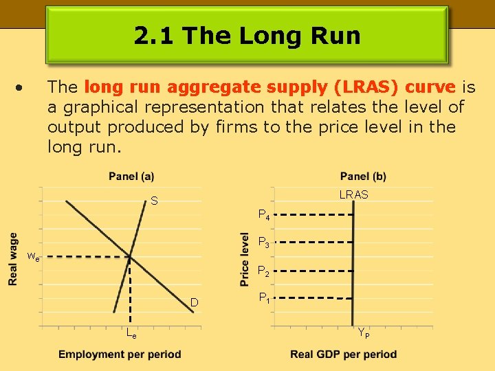
2. 1 The Long Run • The long run aggregate supply (LRAS) curve is a graphical representation that relates the level of output produced by firms to the price level in the long run. LRAS S P 4 P 3 we P 2 D Le P 1 YP

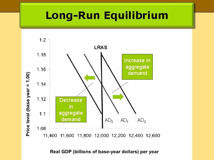
Long-Run Equilibrium LRAS Increase in aggregate demand Decrease in aggregate demand AD 3 AD 1 AD 2

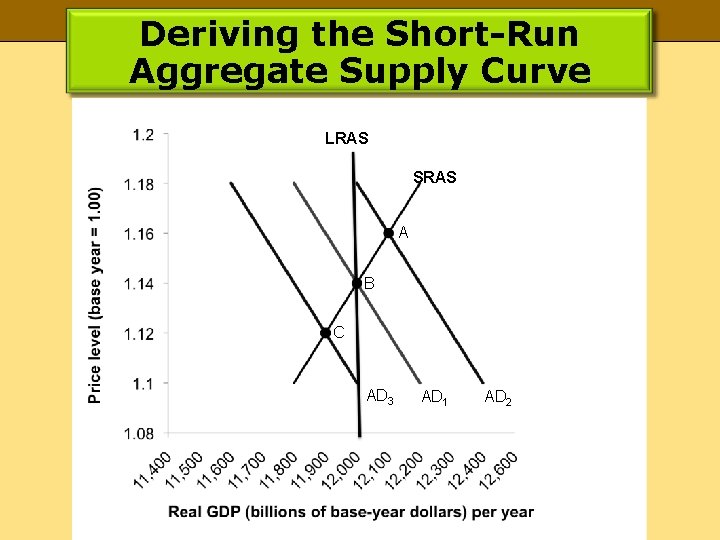
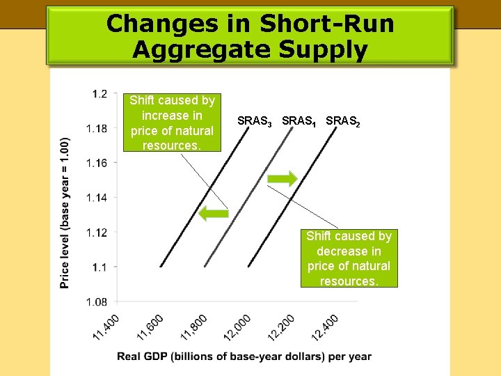
2. 2 The Short Run • • • The short run aggregate supply (SRAS) curve is a graphical representation of the relationship between production and the price level in the short run. A change in the aggregate quantity of goods and services supplied is characterized by movement along the short-run aggregate supply curve. A change in short-run aggregate supply is characterized by a change in the aggregate quantity of goods and services supplied at every price level in the short-run.

Deriving the Short-Run Aggregate Supply Curve LRAS SRAS A B C AD 3 AD 1 AD 2

Changes in Short-Run Aggregate Supply Shift caused by increase in price of natural resources. SRAS 3 SRAS 1 SRAS 2 Shift caused by decrease in price of natural resources.

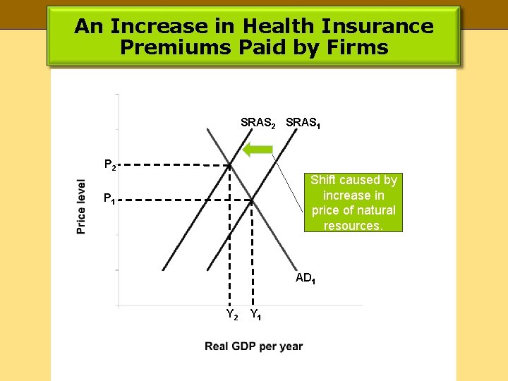
An Increase in Health Insurance Premiums Paid by Firms SRAS 2 SRAS 1 P 2 Shift caused by increase in price of natural resources. P 1 AD 1 Y 2 Y 1

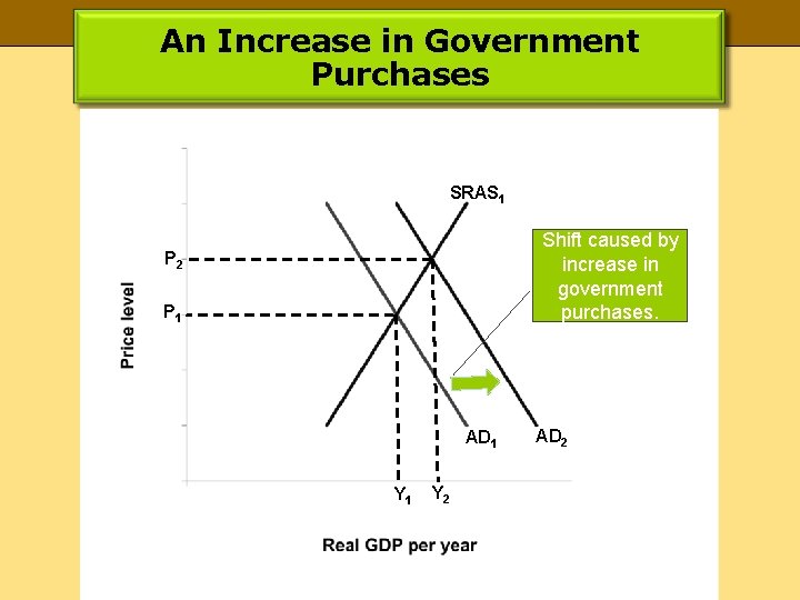
An Increase in Government Purchases SRAS 1 Shift caused by increase in government purchases. P 2 P 1 AD 1 Y 2 AD 2

3. RECESSIONARY AND INFLATIONARY GAPS AND LONG-RUN MACROECONOMIC EQUILIBRIUM Learning Objectives 1. Explain and illustrate graphically recessionary and inflationary gaps and relate these gaps to what is happening in the labor market. 2. Identify the various policy choices available when an economy experiences an inflationary or recessionary gap and discuss some of the pros and cons that make these choices controversial.

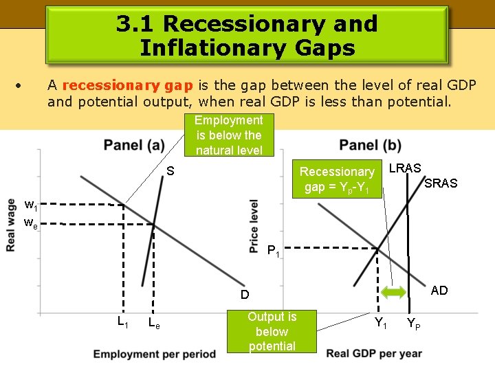
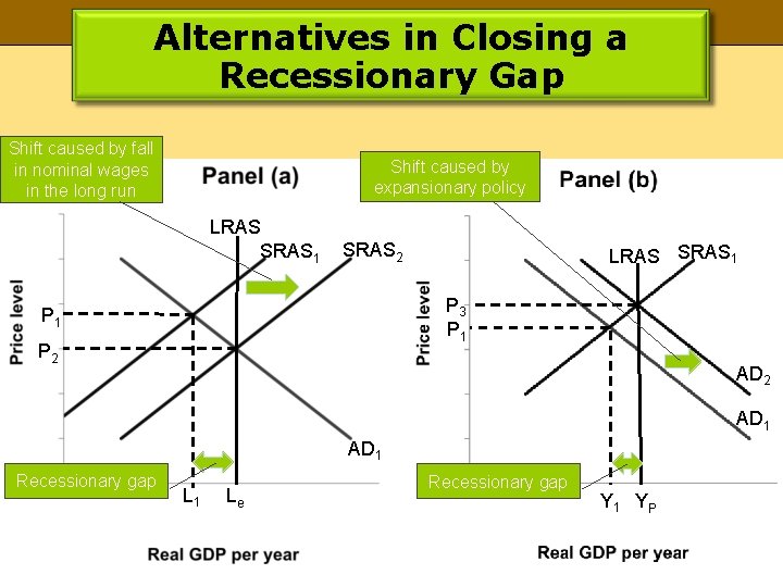
3. 1 Recessionary and Inflationary Gaps • A recessionary gap is the gap between the level of real GDP and potential output, when real GDP is less than potential. Employment is below the natural level S LRAS Recessionary gap = Yp-Y 1 SRAS w 1 we P 1 AD D L 1 Le Output is below potential Y 1 YP

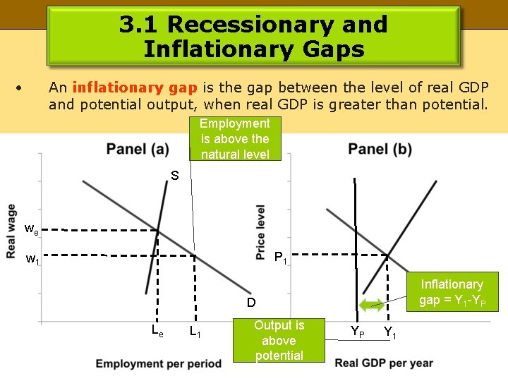
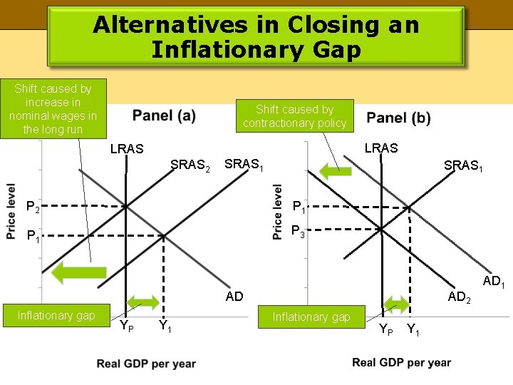
3. 1 Recessionary and Inflationary Gaps • An inflationary gap is the gap between the level of real GDP and potential output, when real GDP is greater than potential. Employment is above the natural level S we P 1 w 1 Inflationary gap = Y 1 -YP D Le L 1 Output is above potential YP Y 1

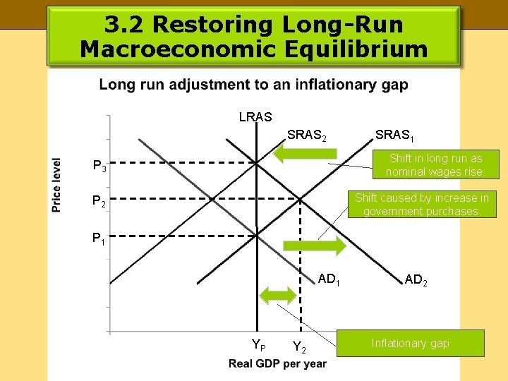
3. 2 Restoring Long-Run Macroeconomic Equilibrium LRAS SRAS 2 SRAS 1 Shift in long run as nominal wages rise. P 3 Shift caused by increase in government purchases. P 2 P 1 AD 1 YP Y 2 AD 2 Inflationary gap

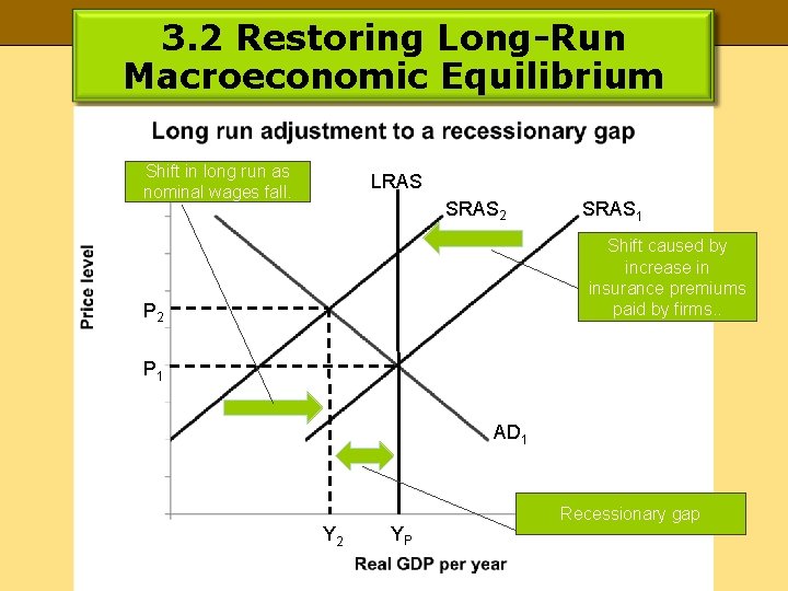
3. 2 Restoring Long-Run Macroeconomic Equilibrium Shift in long run as nominal wages fall. LRAS SRAS 2 SRAS 1 Shift caused by increase in insurance premiums paid by firms. . P 2 P 1 AD 1 Y 2 YP Recessionary gap

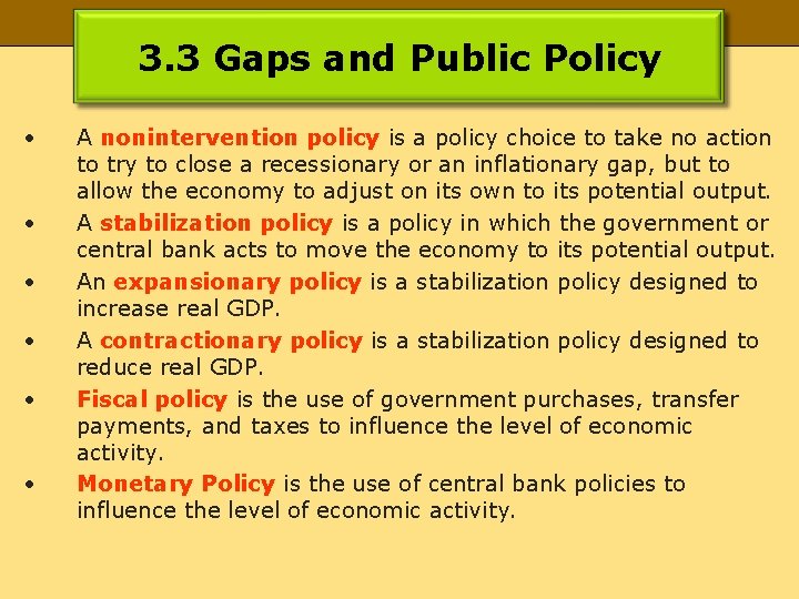
3. 3 Gaps and Public Policy • • • A nonintervention policy is a policy choice to take no action to try to close a recessionary or an inflationary gap, but to allow the economy to adjust on its own to its potential output. A stabilization policy is a policy in which the government or central bank acts to move the economy to its potential output. An expansionary policy is a stabilization policy designed to increase real GDP. A contractionary policy is a stabilization policy designed to reduce real GDP. Fiscal policy is the use of government purchases, transfer payments, and taxes to influence the level of economic activity. Monetary Policy is the use of central bank policies to influence the level of economic activity.

Alternatives in Closing a Recessionary Gap Shift caused by fall in nominal wages in the long run Shift caused by expansionary policy LRAS SRAS 1 SRAS 2 LRAS SRAS 1 P 3 P 1 P 2 AD 1 Recessionary gap L 1 Le Recessionary gap Y 1 YP

Alternatives in Closing an Inflationary Gap Shift caused by increase in nominal wages in the long run Shift caused by contractionary policy LRAS SRAS 2 SRAS 1 P 2 P 1 P 3 AD 2 AD Inflationary gap YP Y 1 AD 1

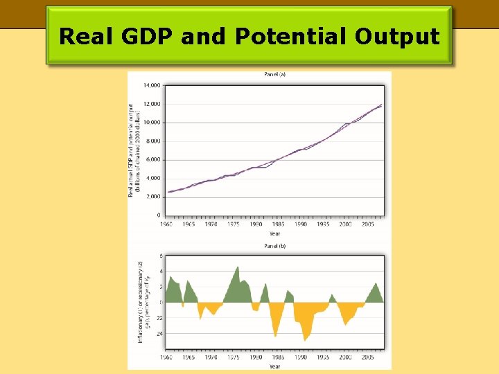
Real GDP and Potential Output