CHAPTER 6 TwoWay Tables Basic Practice of Statistics

CHAPTER 6: Two-Way Tables* Basic Practice of Statistics 7 th Edition Lecture Power. Point Slides

In Chapter 6, We Cover … �Marginal distributions �Conditional distributions �Simpson’s paradox

Categorical Variables �Review: Categorical variables place individuals into one of several groups or categories. �The values of a categorical variable are labels for the different categories. �The distribution of a categorical variable lists the count or percent of individuals who fall into each category. �When a dataset involves two categorical variables, we begin by examining the counts or percents in various categories for one of the variables. Two-way table – Describes two categorical variables, organizing counts according to a row variable and a column variable.

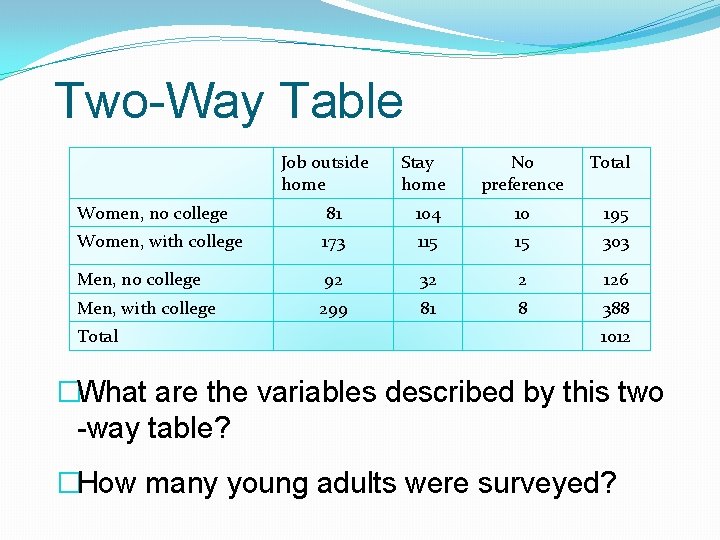
Two-Way Table Job outside home Stay home No preference Total Women, no college 81 104 10 195 Women, with college 173 115 15 303 Men, no college 92 32 2 126 Men, with college 299 81 8 388 Total 1012 �What are the variables described by this two -way table? �How many young adults were surveyed?

Marginal Distribution �The marginal distribution of one of the categorical variables in a two-way table of counts is the distribution of values of that variable among all individuals described by the table. �Note: Percents are often more informative than counts, especially when comparing groups of different sizes. To examine a marginal distribution: 1. Use the data in the table to calculate the marginal distribution (in percents) of the row or column totals. 2. Make a graph to display the marginal distribution.

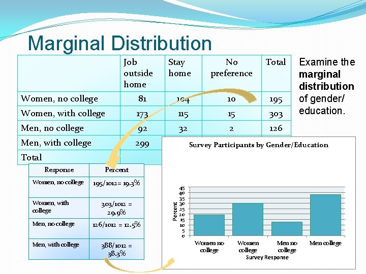
Marginal Distribution Job outside home Stay home No preference Total Examine the marginal distribution of gender/ education. Women, no college 81 104 10 195 Women, with college 173 115 15 303 Men, no college 92 32 2 126 Men, with college 299 81 Survey Participants 8 388 by Gender/Education 1012 Response Percent Women, no college 195/1012= 19. 3% Women, with college Men, no college Men, with college 303/1012 = 29. 9% 126/1012 = 12. 5% 388/1012 = 38. 3% Percent Total 45 40 35 30 25 20 15 10 5 0 Women no college Women Men no college Survey Response Men college

Conditional Distribution �Marginal distributions tell us nothing about the relationship between two variables. �A conditional distribution of a variable describes the values of that variable among individuals who have a specific value of another variable. To examine or compare conditional distributions: �Select the row(s) or column(s) of interest. �Use the data in the table to calculate the conditional distribution (in percents) of the row(s) or column(s). �Make a graph to display the conditional distribution. �Use a side-by-side bar graph or segmented bar graph to compare distributions.

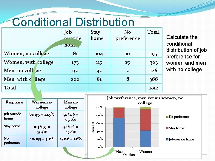
Conditional Distribution Job outside home Stay home No preference Total Women, no college 81 104 10 195 Women, with college 173 115 15 303 Men, no college 92 32 2 126 Men, with college 299 81 8 388 Total 1012 Women no college Men no college Job outside home 81/195 = 41. 5% 92/126 = 73. 0% Stay home 104/195 = 53. 3% 32/126 = 25. 4% 10/195 = 5. 1% 2/126 = 1. 6% No preference, men versus no Job preference, women no women, college Job preference, men versus women, no college 100% 80 60 70 50 60 60% 50 40 40 30 30 40% 20 20 10 10 0 0 20%Job outside home No preference Percent Response Calculate the conditional distribution of job preference for women and men with no college. Job outside home Stay home Men Stay home 0% Men Opinion Women Job outside home Women No preference

Simpson’s Paradox �When studying the relationship between two variables, there may exist a lurking variable that creates a reversal in the direction of the relationship when the lurking variable is ignored, as opposed to the direction of the relationship when the lurking variable is considered. �The lurking variable creates subgroups, and failure to take these subgroups into consideration can lead to misleading conclusions regarding the association between the two variables. An association or comparison that holds for all of several groups can reverse direction when the data are combined to form a single group. This reversal is called Simpson’s paradox.

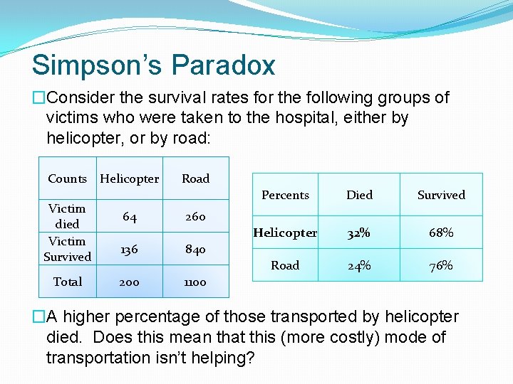
Simpson’s Paradox �Consider the survival rates for the following groups of victims who were taken to the hospital, either by helicopter, or by road: Counts Helicopter Victim died Victim Survived Total 64 136 200 Road Percents Died Survived Helicopter 32% 68% Road 24% 76% 260 840 1100 �A higher percentage of those transported by helicopter died. Does this mean that this (more costly) mode of transportation isn’t helping?

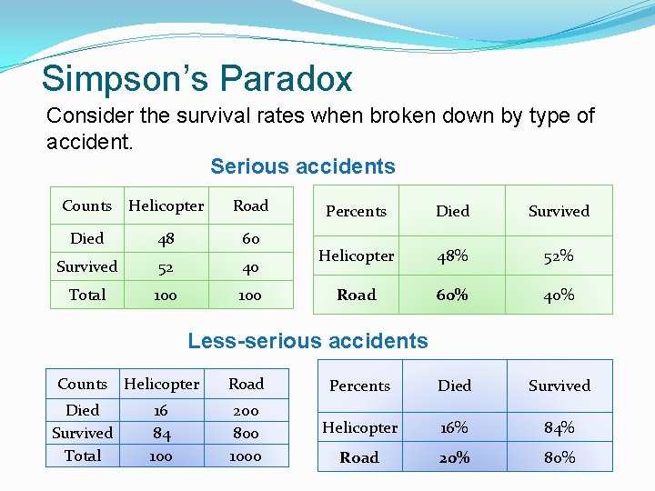
Simpson’s Paradox Consider the survival rates when broken down by type of accident. Serious accidents Counts Helicopter Road Died 48 60 Survived 52 40 Total 100 Percents Died Survived Helicopter 48% 52% Road 60% 40% Less-serious accidents Counts Helicopter Died Survived Total 16 84 100 Road Percents Died Survived 200 800 1000 Helicopter 16% 84% Road 20% 80%

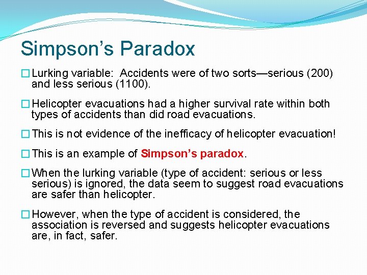
Simpson’s Paradox �Lurking variable: Accidents were of two sorts—serious (200) and less serious (1100). �Helicopter evacuations had a higher survival rate within both types of accidents than did road evacuations. �This is not evidence of the inefficacy of helicopter evacuation! �This is an example of Simpson’s paradox. �When the lurking variable (type of accident: serious or less serious) is ignored, the data seem to suggest road evacuations are safer than helicopter. �However, when the type of accident is considered, the association is reversed and suggests helicopter evacuations are, in fact, safer.