Chapter 6 Section 6 1 Statistics Graphs of

Chapter 6 Section 6. 1 Statistics Graphs of Normal Probability Distributions MR. ZBORIL | MILFORD PEP

Chapter 6 Sect. 6. 1 Graphs of Normal Prob. Distributions You are important to me – don’t ever think otherwise!

Chapter 6 Sect. 6. 1 Graphs of Normal Prob. Distributions Focus Points • Graph a normal curve and summarize its important properties. • Apply the empirical rule to solve real-world problems. • Use control limits to construct control charts. Examine the charts for three possible out-of-control charts.

Chapter 6 Sect. 6. 1 Graphs of Normal Prob. Distributions Focus Points The Denver Post reports the average supermarket shopper spends $20 for every extra 10 minutes they spend in the store, mostly on impulse purchases. It remains in the best interests of the grocery store to keep customers in the store longer. Let x represent the dollar amount of impulse purchases. The mean of the x distribution is $20 and the standard deviation σ is about $7. I’m worth $7 but my kidneys are worth plenty more on the black market!

Chapter 6 Sect. 6. 1 Graphs of Normal Prob. Distributions The σ value controls the spread of the curve. Let’s look at Homework Problem #4. Merry Christmas Margot! Have you finished all your Christmas shopping for your Statistics Teacher, yet?

Chapter 6 Sect. 6. 1 Graphs of Normal Prob. Distributions This Photo by Unknown Author is licensed under CC BY-NC-SA

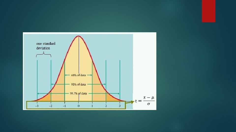
Chapter 6 Sect. 6. 1 Curve Properties Graphs of Normal Probability Distributions Properties of a Normal Curve 1. The curve is bell-shaped with the highest point over the mean μ. 2. The curve is symmetrical about a vertical line through μ. 3. The curve approaches the horizontal axis but never touches it or crosses it. 4. The inflection points, also called transition points, occur above μ + σ and μ – σ. 5. The area under the curve is 1.

Chapter 6 Sect. 6. 1 Example 1 Empirical Rule The playing life of a Sunshine radio is distributed with mean μ = 600 hours and the standard deviation σ = 100 hours. What is the probability that the playing life will be between 600 and 700 hours? Solution: Look at Figure 6 -4 on page 253. We know the mean μ is 600 hours and the standard deviation σ is 100 hours. The probability is equal to the area underneath the curve from μ to μ + σ. From the graph we can see that approx. 34% of the curve’s area falls in the μ to μ + σ range. This tells us the probability a Sunshine radio will last between 600 and 700 hours is about 0. 34.

Chapter 6 Sect. 6. 1 Guided Exercise 2 Empirical Rule The yearly wheat yield per acre on a particular farm is normally distributed with mean μ = 35 bushels and the standard deviation σ = 8 bushels. a) Shade the area under the curve in Figure 6 -5 (next slide) that represents the probability that an acre will yield between 19 and 35 bushels. b) Is the area the same as the area between μ -2σ and μ?

Chapter 6 Sect. 6. 1 Guided Exercise 2 Empirical Rule Guided Exercise 2 Figure 6 -5 0, 06 mean μ = 35 0, 05 standard deviation σ = 8 0, 04 0, 03 0, 02 μ + 2σ μ - 2σ 0, 01 μ - 3σ μ-σ μ μ+σ 31 35 39 Bushels of Wheat 43 μ + 3σ 0 7 11 15 19 23 27 47 51 55 59 63

Chapter 6 Sect. 6. 1 Guided Exercise 2 Empirical Rule Guided Exercise 2 Figure 6 -6 0, 06 mean μ = 35 0, 05 standard deviation σ = 8 0, 04 0, 03 0, 02 μ + 2σ μ - 2σ 0, 01 μ - 3σ μ-σ μ μ+σ 31 35 39 Bushels of Wheat 43 μ + 3σ 0 7 11 15 19 23 27 47 51 55 59 63

Chapter 6 Sect. 6. 1 Guided Exercise 2 Empirical Rule The yearly wheat yield per acre on a particular farm is normally distributed with mean μ = 35 bushels and the standard deviation σ = 8 bushels. a) Shade the area under the curve in Figure 6 -5 (next slide) that represents the probability that an acre will yield between 19 and 35 bushels. b) Is the area the same as the area between μ -2σ and μ? c) Use figure 6 -3 to find the percentage of area over the interval between 19 and 35. The answer is 47. 5% d) What is the probability that the yield will be between 19 and 35 bushels per acre? Since the area underneath the curve = 1 and the shaded area represents 47. 5% of the total area, the probability is 0. 475.

Chapter 6 Sect. 6. 1 Control Charts are useful for examining data for: a) equally-spaced time intervals or b) sequential order. Examples of sequential order data include: a) sugar content of bottled drinks taken sequentially off a production line b) clerical errors in a bank from day-to-day c) advertising expenses from month-to-month d) new customers from year-to-year Any business manager or production supervisor will tell you there is a degree of variability in a - d above.

Chapter 6 Sect. 6. 1 Control Charts HOW TO MAKE A CONTROL CHART FOR THE RANDOM VARIABLE x A control chart for a random variable x is a plot of observed x values in time sequence order. 1. Find the mean μ and standard deviation σ of the x distribution by using past data from a period when the process was “in-control” or b) using specified “target” values for μ and σ. a) 2. Create a graph in which the vertical axis represents x values and the horizontal axis represents time. 3. Draw a horizontal line at height μ and horizontal, dashed control-limit lines at μ + 2σ and μ + 3σ. 4. Plot the variable x on the graph line in time sequence order. Use line segments to connect the point in time sequence order.

Chapter 6 Sect. 6. 1 Example 2 pg. 255 Control Charts Susan Tamara is director of personnel at the Antlers Lodge in Denali National Park, Alaska. Every summer Ms. Tamara hires many part-time employees from all over the United States. Most are college students seeking summer employment. One of the primary responsibilities of the employees is making up the rooms. The rooms are to be ready by 3: 30 pm. Every 15 days Ms. Tamara has a staff meeting and shows a control chart for the number of rooms not made up by 3: 30 pm. From previous data, she knows the mean μ = 19. 3 rooms not made up and the standard deviation σ = 4. 7 rooms.

Chapter 6 Sect. 6. 1 Example 2 pg. 255 Table 6 -1 shows the number of rooms not made up by 3: 30 pm for the last 15 days. Day 1 2 3 4 5 6 7 8 9 10 11 12 13 14 15 x 11 20 25 23 16 19 8 25 17 20 23 29 18 14 10 The next slide shows Ms. Tamara’s control chart. Note the lines placed at the mean μ (19. 3 days) along with the μ + 2σ points 19. 3 + 9. 4 = 28. 70 & 19. 3 – 9. 4 = 9. 90 and μ + 3σ points 19. 3 + 14. 1 = 33. 40 & 19. 3 – 14. 1 = 5. 20

Section 6. 1 Control Charts 35 μ + 3σ 30 20 Rooms 25 29 25 μ + 2σ 33. 40 28. 70 25 23 23 20 20 19 17 16 15 μ 18 19. 30 14 11 10 10 μ - 2σ 8 5 9. 90 μ - 3σ 0 0 1 2 3 4 5 6 7 8 9 10 11 12 13 Day 14 15 5. 20

Chapter 6 Sect. 6. 1 Control Charts – Out of Control Signals 1. Signal I : One point falls beyond the 3σ level. Through the Empirical rule we know the probability a point lies within 3σ is 0. 997. The probability that Signal 1 is a false alarm is 1 – 0. 997 or 0. 003. 2. Signal II : A run of nine consecutive points on one side of the center line (target value μ). There is a 50% chance the x values will lie above or below the centerline. The probability of nine consecutive runs is (0. 5)9 or 0. 002. If we consider both sides the probability becomes 0. 004. The probability that Signal II is a false alarm is 0. 004.

Chapter 6 Sect. 6. 1 Control Charts – Out of Control Signals 3. Signal III : At least two of three consecutive points lie beyond the 2σ level on the same side of the center line Through the Empirical rule the probability that an x value will be above the 2σ level is about 0. 023. Using the binomial probability distribution (success would be a value outside 2σ), the probability of two or more successes out of three trials is 3 n. Cr 2 (. 023)2 (. 997) + 3 n. Cr 3 (. 023)3 (. 997)0 ≈ 0. 002. If we consider both sides the probability becomes 0. 004. The probability that Signal II is a false alarm is 0. 004.

Chapter 6 Sect. 6. 1 Guided Exercise 3 Figures 6 -8 and 6 -9 on the next slides show control charts for two other 15 -day periods.

Section 6. 1 Control Charts Figure 6 -8 Report II 35 μ + 3σ 25 20 30 Rooms 30 27 26 28 27 23 μ + 2σ 26 33. 40 28. 70 23 21 21 20 μ 19. 30 17 15 15 10 10 μ - 2σ 6 5 μ - 3σ 0 0 1 2 3 4 5 6 7 8 9 10 11 12 13 Day 14 15 9. 90 5. 20

Section 6. 1 Control Charts Figure 6 -9 Report III 35 34 25 20 30 μ + 2σ Rooms 30 μ + 3σ 33. 40 28. 70 23 21 21 20 19 18 μ 19 19. 30 15 12 12 11 10 12 8 6 5 μ - 3σ 0 0 1 2 3 4 5 6 7 8 9 10 11 12 μ - 2σ 13 Day 14 15 9. 90 5. 20

Section 6. 1 Homework Problem 15 a Visitors Treated at YPMS 40 35 30 30 25 25 24 20 19 20 23 19 17 16 15 15 10 0 1 2 3 4 5 6 7 8 9 10 11

Section 6. 1 Homework Problem 15 a Visitors Treated at YPMS 40 36 35 37 35 32 30 28 24 25 21 20 20 15 15 12 10 0 1 2 3 4 5 6 7 8 9 10 11

Section 6. 1 Normal Curves and Sampling Distribution Questions?

Chapter 6 Section 6. 2 Statistics Standard Units and Areas Under the Standard Normal Distribution MR. ZBORIL | MILFORD PEP

Chapter 6 Sect. 6. 2 Graphs of Normal Prob. Distributions You are important to me – don’t ever think otherwise!

Chapter 6 Sect. 6. 2 Standard Units and Areas Under the Standard Normal Distribution Focus Points • Given μ and σ, convert raw data to z scores. • Given μ and σ, convert z scores to raw data. • Graph the standard normal distribution, and find areas under the standard normal curve.

Chapter 6 Sect. 6. 2 z Scores and Raw Scores Tina and Jack are in two different sections of the same course. Each section is large and the midterm grades followed a normal distribution. Tina’s section has an average (mean) of 64. Tina scored a 74. Jack’s section has an average (mean) of 72. Jack scored an 82. Both were happy they scored 10 points above their section mean, but neither score really tells us how they performed with respect to the other students.

Chapter 6 Sect. 6. 2 z Scores and Raw Scores We will begin using a new measurement that tells us the number of standard deviations between the x value and the μ mean. This is called the z value or z score. Looking at a graph, this is a measure of distance. Number of standard deviations between the measurement and the mean. = Difference between the measurement and the mean. Standard deviation

Chapter 6 Sect. 6. 2 z Scores and Raw Scores

Chapter 6 Sect. 6. 2 z Scores and Raw Scores x Value in Original Distribution Corresponding z Value or Standard Unit x=μ z=0 x>μ z>0 x<μ z<0 Hello Class!

Chapter 6 Sect. 6. 2 Example 4 A pizza parlor franchise specifes that the average (mean) amount of cheese on a large pizza should be 8 ounces and the standard deviation only 0. 5 ounces. An inspector picks out a large pizza at random and finds it only has 6. 9 ounces of cheese. Assume that the amount of cheese on a pizza follows a normal distribution. If the amount of cheese is below the mean by more than 3 standard deviations, the parlor will be in danger of losing its franchise. How many standard deviations from the mean is 6. 9? Is the pizza parlor in danger of losing its franchise?

Chapter 6 Sect. 6. 2 Example 4 If the original distribution of the x values is normal, the corresponding z values will have a normal distribution as well. The z distribution has a mean of 0 and a standard deviation of 1. This graph has a special name – the Standard Normal Deviation.

Chapter 6 Sect. 6. 2 Standard Normal Distribution

Chapter 6 Sect. 6. 2 Standard Normal Distribution Why do we invest so much time into creating these graphs? There are extensive tables that show the area underneath the standard normal curve for almost any interval along the z axis. These areas are important because each area is equal to the probability that the measurement of the item selected falls within the interval. If the original distribution of the x values is normal, the corresponding z values will have a normal distribution as well. The z distribution has a mean of 0 and a standard deviation of 1. This graph has a special name – the Standard Normal Deviation.

Chapter 6 Sect. 6. 2 Standard Normal Distribution HOW TO USE A LEFT-TAIL STYLE STANDARD NORMAL DISTRIBUTION TABLE 1. For areas to the left of a specified z value, use the table entry directly. 2. For areas to the right of a specified z value, look up the table entry for z and subtract the area from 1. 3. For areas between two z values, z 1 and z 2 (where z 2 > z 1), subtract the table area for z 1, from the table area for z 2.

Chapter 6 Sect. 6. 2 Using Table 5 of Appendix 2 This is summarized at the top of pg. 272 To find the following: Do the following: (a) Area to the left of a z value Use Table 5 of Appendix II directly (b) Area to the right of a z value Area underneath the entire curve (1. 000) - Area to the left of z. (c) Area to the right of a z value Find the area to the left of –z. (d) Area between two z values Area to the left of z 2 - area to the left of z 1

Chapter 6 Sect. 6. 2 Example 6 pg. 272 -273 Example 6 Using Table to Find Areas Use Table 5 of Appendix II to find the specified areas. a) Find the area between z = 1. 00 and z = 2. 70. Solution : First sketch a diagram showing the area. Because we are finding the area between two z values, we subtract corresponding table entries.

Chapter 6 Sect. 6. 2 Example 6 pg. 273 Solution for part A Example 6 Figure 6 -19 2. 70 -3 -2 -1 0 1 2 3 (Area between 1. 00 and 2. 70) = (Area to the left of 2. 70) – (Area left of 1. 00) = 0. 9965 – 0. 8413 = 0. 1552

Chapter 6 Sect. 6. 2 Example 6 pg. 273 Solution for part B Example 6 Figure 6 -19 -3 -2 -1 0 1 2 3 (Area to the right of z = 0. 94) = (Area under the entire curve) – (Area to the left of 0. 94) = 1. 000 – 0. 8264 = 0. 1736

Section 6. 2 Areas Under the Standard Normal Distribution Questions?