Chapter 6 Searching trees and more Sorting Algorithms

Chapter 6: Searching trees and more Sorting Algorithms 6. 1 Binnary Tree The Bin Tree class with traversing methods 6. 2 Searching Trees 6. 2. 1 AVL Trees 6. 3 Heap. Sort and Bucket. Sort 6. 3. 1 Heap. Sort 6. 3. 2 Bucket. Sort 1

6. 1 Binary trees (Continuation) Characteristics: • Maximal height of a binary tree with n nodes is n -1. (this is when each internal node has exactly one child, this is in fact a linear linked list. ) • Minimal number of nodes in a binary tree of height h is h+1. (Ditto) 2

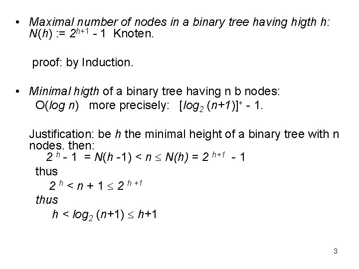
• Maximal number of nodes in a binary tree having higth h: N(h) : = 2 h+1 - 1 Knoten. proof: by Induction. • Minimal higth of a binary tree having n b nodes: O(log n) more precisely: [log 2 (n+1)]+ - 1. Justification: be h the minimal height of a binary tree with n nodes. then: 2 h - 1 = N(h -1) < n N(h) = 2 h+1 - 1 thus 2 h < n + 1 2 h +1 thus h < log 2 (n+1) h+1 3

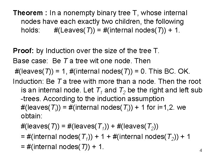
Theorem : In a nonempty binary tree T, whose internal nodes have each exactly two children, the following holds: #(Leaves(T)) = #(internal nodes(T)) + 1. Proof: by Induction over the size of the tree T. Base case: Be T a tree wit one node. Then #(leaves(T)) = 1, #(internal nodes(T)) = 0. This BC. OK. Induction: Be T a tree with more than a node. Then the root is an internal node. Let T 1 and T 2 be the right and left sub -trees. According to the induction assumption #(leaves(Ti)) = #(internal nodes(Ti)) + 1 for i=1, 2. we obtain: #(leaves(T)) = #(leaves(T 1)) + #(leaves(T 2)) = #(internal nodes(T 1)) + 1 + #(internal nodes(T 2)) + 1 = #(internal nodes(T)) + 1. 4

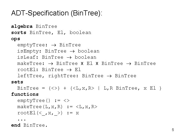
ADT-Specification (Bin. Tree): algebra Bin. Tree sorts Bin. Tree, El, boolean ops empty. Tree: Bin. Tree is. Empty: Bin. Tree boolean is. Leaf: Bin. Tree boolean make. Tree: Bin. Tree x El x Bin. Tree root. El: Bin. Tree El left. Tree, right. Tree: Bin. Tree sets Bin. Tree = {<>} + {<L, x, R> | L, R Bin. Tree, x El } functions empty. Tree() : = <> make. Tree(L, x, R) : = <L, x, R> root. El(<_, x, _>) : = x. . . end Bin. Tree. 5

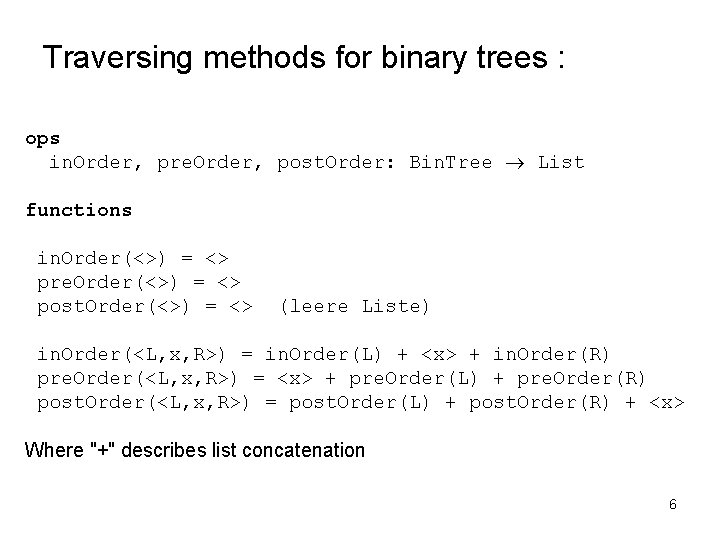
Traversing methods for binary trees : ops in. Order, pre. Order, post. Order: Bin. Tree List functions in. Order(<>) = <> pre. Order(<>) = <> post. Order(<>) = <> (leere Liste) in. Order(<L, x, R>) = in. Order(L) + <x> + in. Order(R) pre. Order(<L, x, R>) = <x> + pre. Order(L) + pre. Order(R) post. Order(<L, x, R>) = post. Order(L) + post. Order(R) + <x> Where "+" describes list concatenation 6

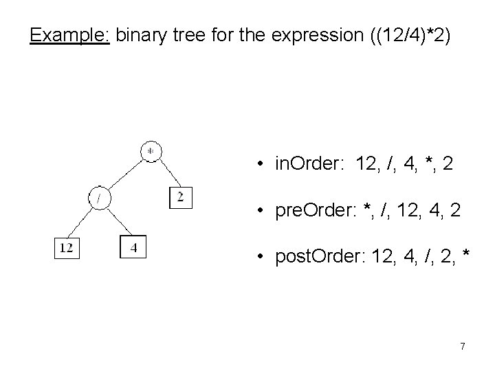
Example: binary tree for the expression ((12/4)*2) • in. Order: 12, /, 4, *, 2 • pre. Order: *, /, 12, 4, 2 • post. Order: 12, 4, /, 2, * 7

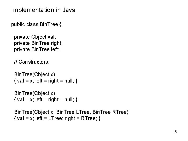
Implementation in Java public class Bin. Tree { private Object val; private Bin. Tree right; private Bin. Tree left; // Constructors: Bin. Tree(Object x) { val = x; left = right = null; } Bin. Tree(Object x, Bin. Tree LTree, Bin. Tree RTree) { val = x; left = LTree; right = RTree; } 8

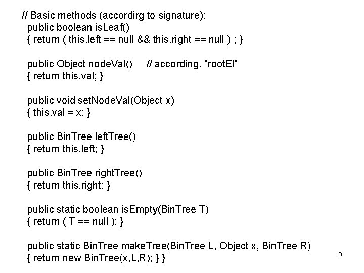
// Basic methods (accordirg to signature): public boolean is. Leaf() { return ( this. left == null && this. right == null ) ; } public Object node. Val() // according. "root. El" { return this. val; } public void set. Node. Val(Object x) { this. val = x; } public Bin. Tree left. Tree() { return this. left; } public Bin. Tree right. Tree() { return this. right; } public static boolean is. Empty(Bin. Tree T) { return ( T == null ); } public static Bin. Tree make. Tree(Bin. Tree L, Object x, Bin. Tree R) { return new Bin. Tree(x, L, R); } } 9

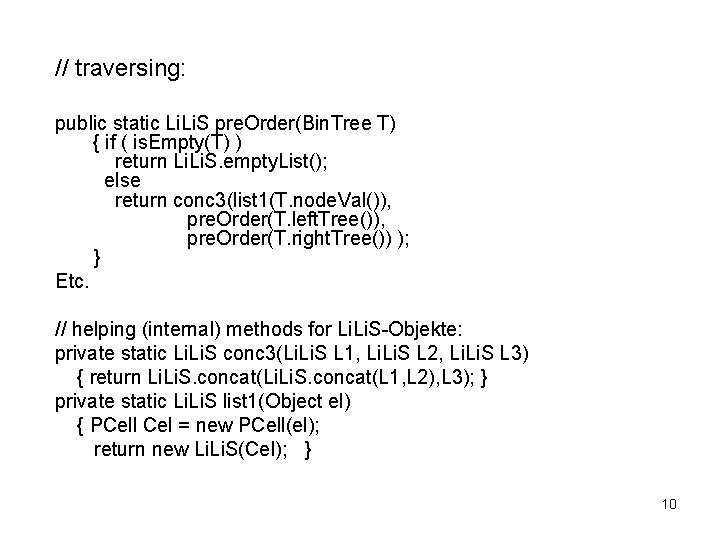
// traversing: public static Li. S pre. Order(Bin. Tree T) { if ( is. Empty(T) ) return Li. S. empty. List(); else return conc 3(list 1(T. node. Val()), pre. Order(T. left. Tree()), pre. Order(T. right. Tree()) ); } Etc. // helping (internal) methods for Li. S-Objekte: private static Li. S conc 3(Li. S L 1, Li. S L 2, Li. S L 3) { return Li. S. concat(Li. S. concat(L 1, L 2), L 3); } private static Li. S list 1(Object el) { PCell Cel = new PCell(el); return new Li. S(Cel); } 10

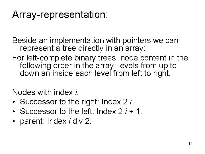
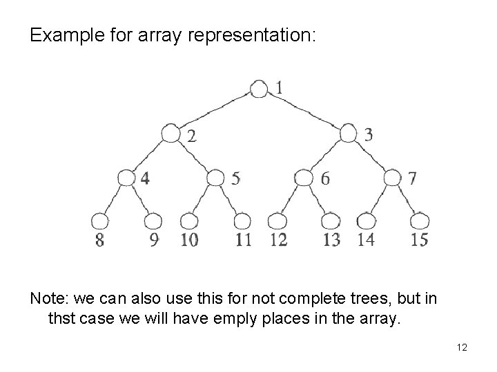
Array-representation: Beside an implementation with pointers we can represent a tree directly in an array: For left-complete binary trees: node content in the following order in the array: levels from up to down an inside each level frpm left to right. Nodes with index i: • Successor to the right: Index 2 i. • Successor to the left: Index 2 i + 1. • parent: Index i div 2. 11

Example for array representation: Note: we can also use this for not complete trees, but in thst case we will have emply places in the array. 12

Generalization for not binary trees: A possible definition: Definition: a tree. T is a tuple T = ( x, T 1 , . . . , Tk ), where x is a valid content for the node and Ti are trees. Here k = 0 is also valid. The corresponding trivial tree is composed by only one node. (However: with this approach belongs a null not to the set of trees!) 13

Descriptions and Characteristics: • Grade of a node: number of children. • Grade of a tree T: grade(T) = max { grade(k) | k nodes in T } • The maximal number of elements in a tree of height h and grade d is N(h) = (d h+1 - 1) / (d - 1). 14

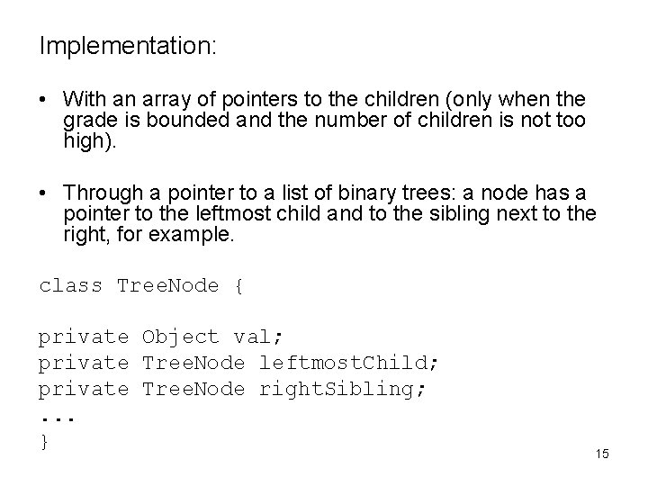
Implementation: • With an array of pointers to the children (only when the grade is bounded and the number of children is not too high). • Through a pointer to a list of binary trees: a node has a pointer to the leftmost child and to the sibling next to the right, for example. class Tree. Node { private Object val; private Tree. Node leftmost. Child; private Tree. Node right. Sibling; . . . } 15

6. 2 Search trees Dictionary-Operations: • member • insert • delete Goal: implement these efficiently 16

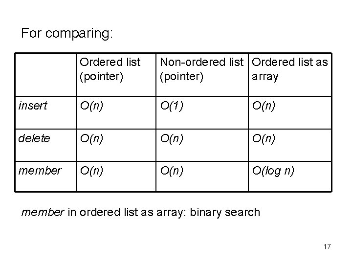
For comparing: Ordered list (pointer) Non-ordered list Ordered list as (pointer) array insert O(n) O(1) O(n) delete O(n) member O(n) O(log n) member in ordered list as array: binary search 17

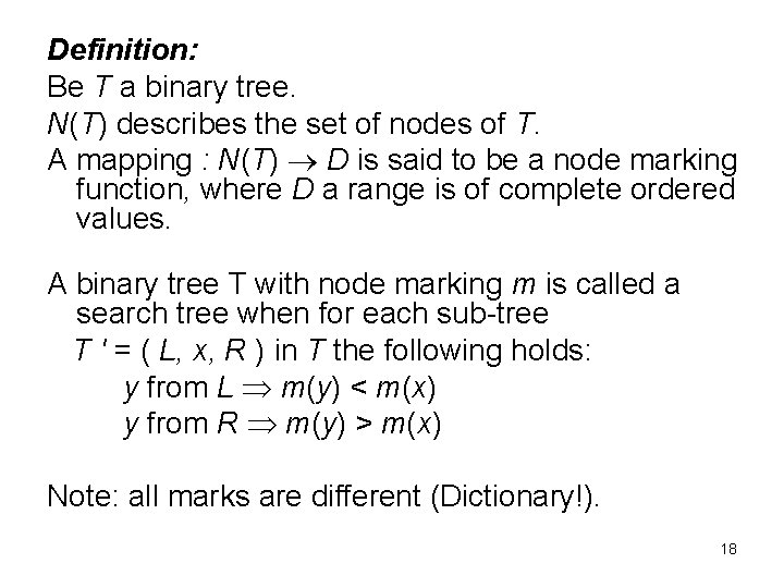
Definition: Be T a binary tree. N(T) describes the set of nodes of T. A mapping : N(T) D is said to be a node marking function, where D a range is of complete ordered values. A binary tree T with node marking m is called a search tree when for each sub-tree T ' = ( L, x, R ) in T the following holds: y from L m(y) < m(x) y from R m(y) > m(x) Note: all marks are different (Dictionary!). 18

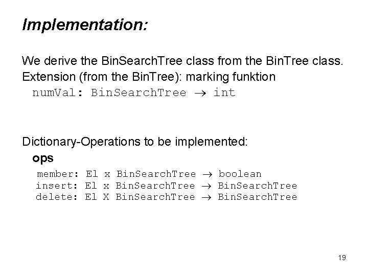
Implementation: We derive the Bin. Search. Tree class from the Bin. Tree class. Extension (from the Bin. Tree): marking funktion num. Val: Bin. Search. Tree int Dictionary-Operations to be implemented: ops member: El x Bin. Search. Tree boolean insert: El x Bin. Search. Tree delete: El X Bin. Search. Tree 19

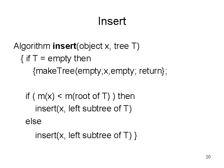
Insert Algorithm insert(object x, tree T) { if T = empty then {make. Tree(empty, x, empty; return}; if ( m(x) < m(root of T) ) then insert(x, left subtree of T) else insert(x, left subtree of T) } 20

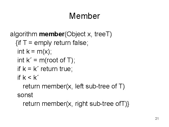
Member algorithm member(Object x, tree. T) {if T = emply return false; int k = m(x); int k´ = m(root of T); if k = k´ return true; if k < k´ return member(x, left sub-tree of T) sonst return member(x, right sub-tree of. T)} 21

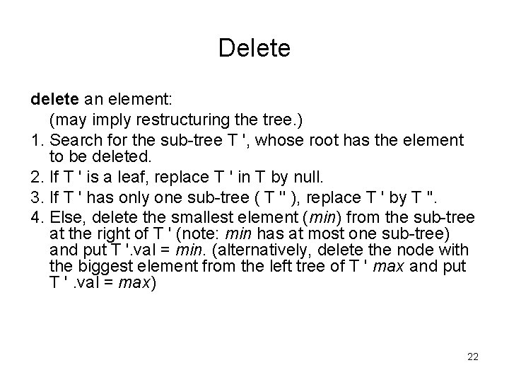
Delete delete an element: (may imply restructuring the tree. ) 1. Search for the sub-tree T ', whose root has the element to be deleted. 2. If T ' is a leaf, replace T ' in T by null. 3. If T ' has only one sub-tree ( T '' ), replace T ' by T ''. 4. Else, delete the smallest element (min) from the sub-tree at the right of T ' (note: min has at most one sub-tree) and put T '. val = min. (alternatively, delete the node with the biggest element from the left tree of T ' max and put T '. val = max) 22

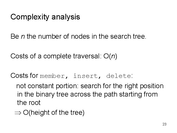
Complexity analysis Be n the number of nodes in the search tree. Costs of a complete traversal: O(n) Costs for member, insert, delete: not constant portion: search for the right position in the binary tree across the path starting from the root O(height of the tree) 23

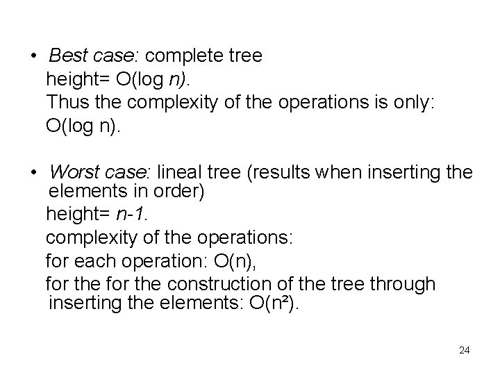
• Best case: complete tree height= O(log n). Thus the complexity of the operations is only: O(log n). • Worst case: lineal tree (results when inserting the elements in order) height= n-1. complexity of the operations: for each operation: O(n), for the construction of the tree through inserting the elements: O(n²). 24

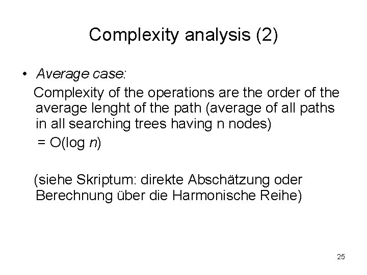
Complexity analysis (2) • Average case: Complexity of the operations are the order of the average lenght of the path (average of all paths in all searching trees having n nodes) = O(log n) (siehe Skriptum: direkte Abschätzung oder Berechnung über die Harmonische Reihe) 25

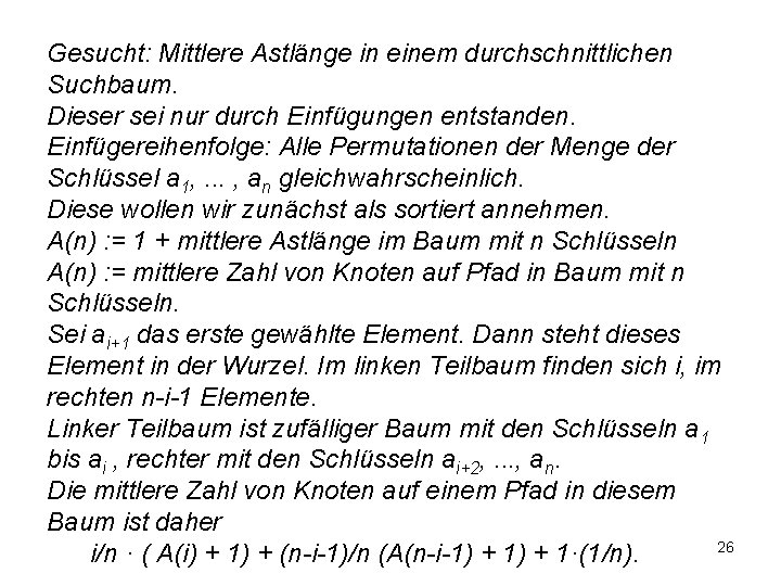
Gesucht: Mittlere Astlänge in einem durchschnittlichen Suchbaum. Dieser sei nur durch Einfügungen entstanden. Einfügereihenfolge: Alle Permutationen der Menge der Schlüssel a 1, . . . , an gleichwahrscheinlich. Diese wollen wir zunächst als sortiert annehmen. A(n) : = 1 + mittlere Astlänge im Baum mit n Schlüsseln A(n) : = mittlere Zahl von Knoten auf Pfad in Baum mit n Schlüsseln. Sei ai+1 das erste gewählte Element. Dann steht dieses Element in der Wurzel. Im linken Teilbaum finden sich i, im rechten n-i-1 Elemente. Linker Teilbaum ist zufälliger Baum mit den Schlüsseln a 1 bis ai , rechter mit den Schlüsseln ai+2, . . . , an. Die mittlere Zahl von Knoten auf einem Pfad in diesem Baum ist daher 26 i/n · ( A(i) + 1) + (n-i-1)/n (A(n-i-1) + 1·(1/n).

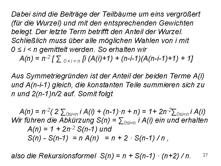
Dabei sind die Beiträge der Teilbäume um eins vergrößert (für die Wurzel) und mit den entsprechenden Gewichten belegt. Der letzte Term betrifft den Anteil der Wurzel. Schließlich muss über alle möglichen Wahlen von i mit 0 ≤ i < n gemittelt werden. So erhalten wir A(n) = n-2 [ ∑ 0 ≤ i < n [i (A(i)+1) + (n-i-1)(A(n-i-1)+1) + 1] Aus Symmetriegründen ist der Anteil der beiden Terme A(i) und A(n-i-1) gleich, die konstanten Teile summieren sich zu n und 2(n-1)n/2 auf. Somit folgt A(n) = n-2( 2 ∑ 0≤i<n i A(i) + (n-1)·n + n) = 1+ 2 n-2∑ 0≤i<n i A(i) Wir führen die Abkürzung S(n) = ∑ 0≤i<n i A(i) ein und erhalten A(n) = 1 + 2 n-2 S(n-1) und S(n) - S(n-1) = n A(n) = n + 2 · S(n-1) / n , also die Rekursionsformel S(n) = n + S(n-1) · (n+2) / n. 27

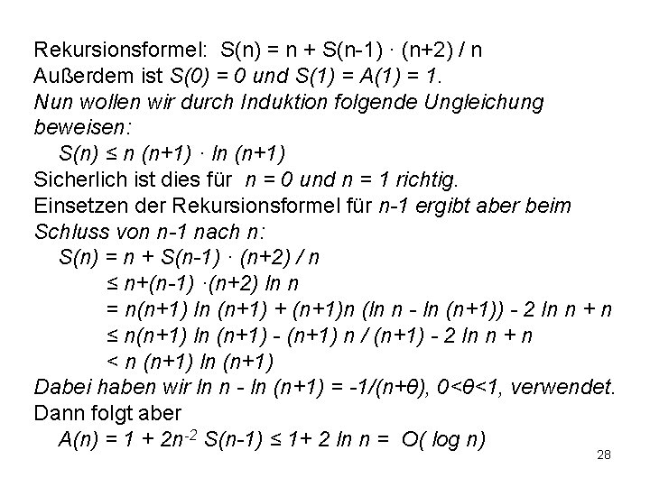
Rekursionsformel: S(n) = n + S(n-1) · (n+2) / n Außerdem ist S(0) = 0 und S(1) = A(1) = 1. Nun wollen wir durch Induktion folgende Ungleichung beweisen: S(n) ≤ n (n+1) · ln (n+1) Sicherlich ist dies für n = 0 und n = 1 richtig. Einsetzen der Rekursionsformel für n-1 ergibt aber beim Schluss von n-1 nach n: S(n) = n + S(n-1) · (n+2) / n ≤ n+(n-1) ·(n+2) ln n = n(n+1) ln (n+1) + (n+1)n (ln n - ln (n+1)) - 2 ln n + n ≤ n(n+1) ln (n+1) - (n+1) n / (n+1) - 2 ln n + n < n (n+1) ln (n+1) Dabei haben wir ln n - ln (n+1) = -1/(n+θ), 0<θ<1, verwendet. Dann folgt aber A(n) = 1 + 2 n-2 S(n-1) ≤ 1+ 2 ln n = O( log n) 28

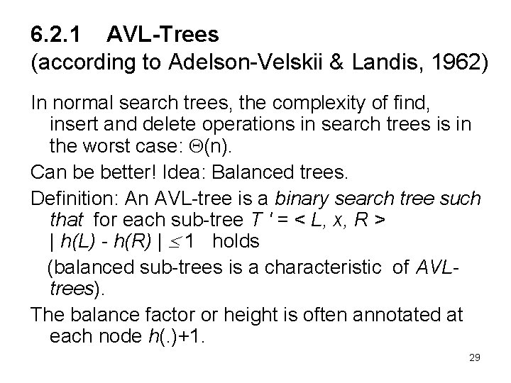
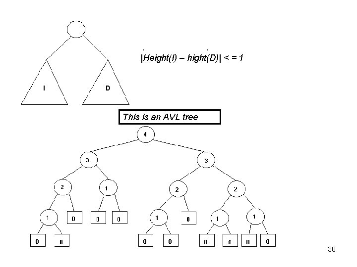
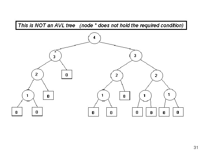
6. 2. 1 AVL-Trees (according to Adelson-Velskii & Landis, 1962) In normal search trees, the complexity of find, insert and delete operations in search trees is in the worst case: (n). Can be better! Idea: Balanced trees. Definition: An AVL-tree is a binary search tree such that for each sub-tree T ' = < L, x, R > | h(L) - h(R) | 1 holds (balanced sub-trees is a characteristic of AVLtrees). The balance factor or height is often annotated at each node h(. )+1. 29

|Height(I) – hight(D)| < = 1 This is an AVL tree 30

This is NOT an AVL tree (node * does not hold the required condition) 31

Goals 1. How can the AVL-characteristics be kept when inserting and deleting nodes? 2. We will see that for AVL-trees the complexity of the operations is in the worst case = O(height of the AVL-tree) = O(log n) 32

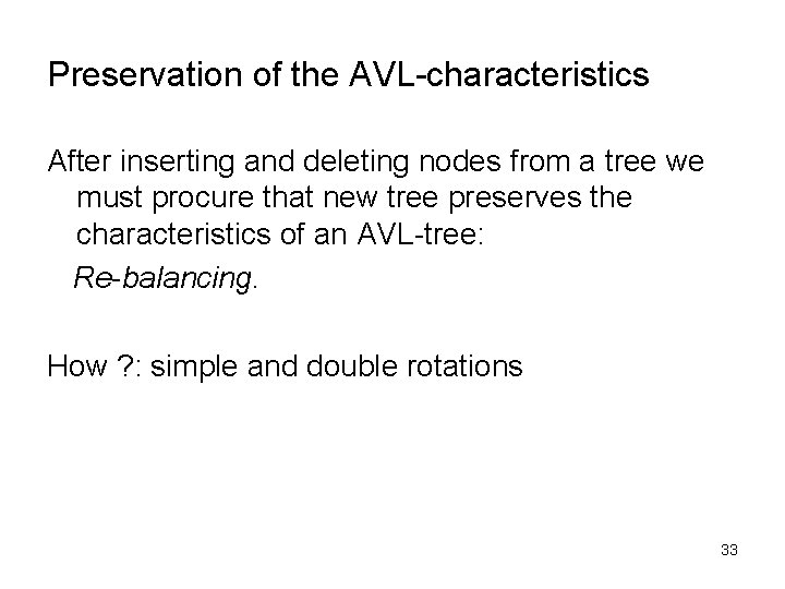
Preservation of the AVL-characteristics After inserting and deleting nodes from a tree we must procure that new tree preserves the characteristics of an AVL-tree: Re-balancing. How ? : simple and double rotations 33

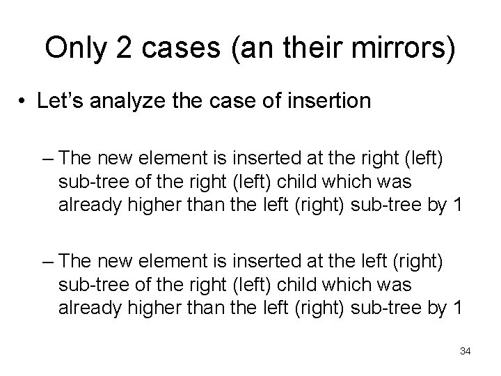
Only 2 cases (an their mirrors) • Let’s analyze the case of insertion – The new element is inserted at the right (left) sub-tree of the right (left) child which was already higher than the left (right) sub-tree by 1 – The new element is inserted at the left (right) sub-tree of the right (left) child which was already higher than the left (right) sub-tree by 1 34

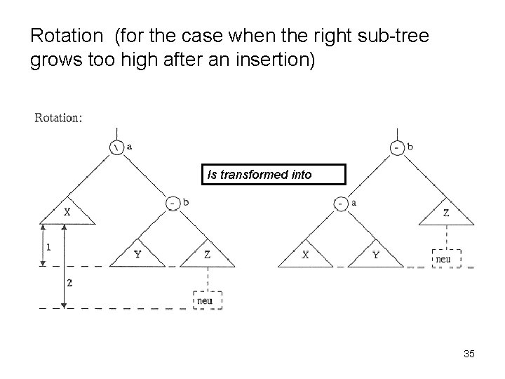
Rotation (for the case when the right sub-tree grows too high after an insertion) Is transformed into 35

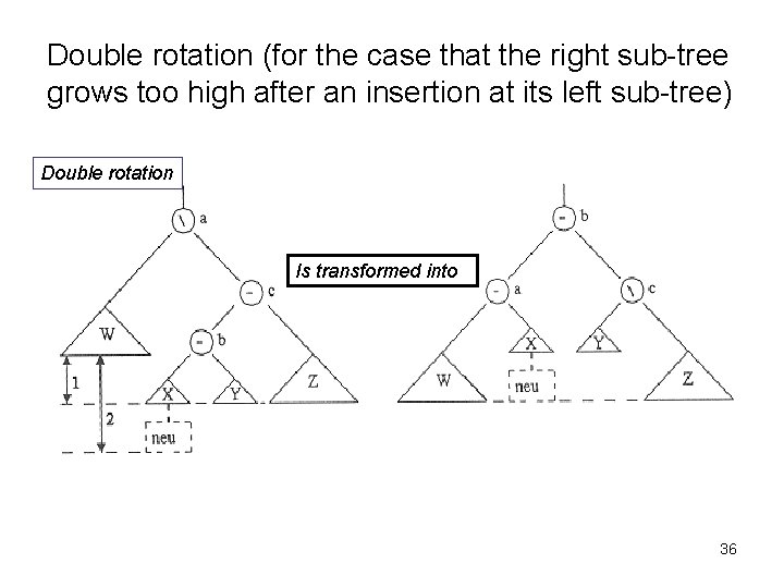
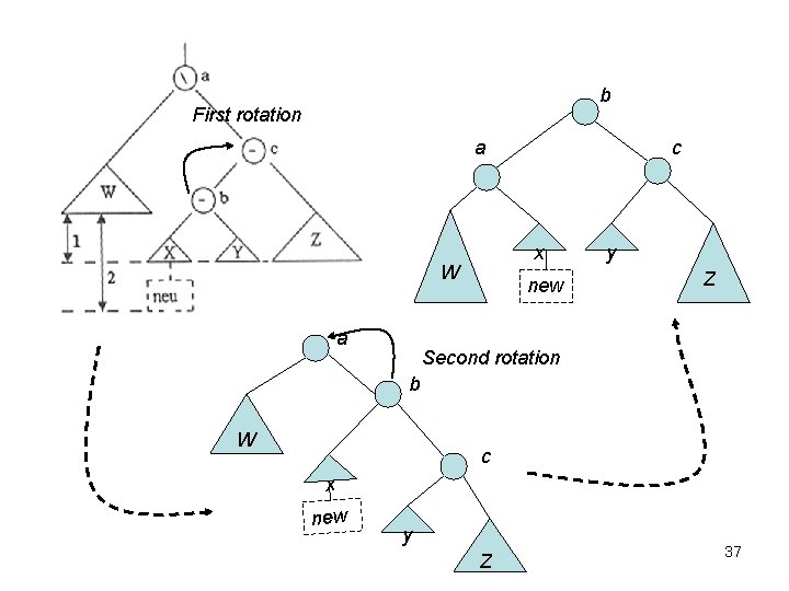
Double rotation (for the case that the right sub-tree grows too high after an insertion at its left sub-tree) Double rotation Is transformed into 36

b First rotation a x W a c new y Z Second rotation b W c x new y Z 37

Re-balancing after insertion: After an insertion the tree might be still balanced or: theorem: After an insertion we need only one rotation of double-rotation at the first node that got unbalanced * in order to re-establish the balance properties of the AVL tree. (* : on the way from the inserted node to the root). Because: after a rotation or double rotation the resulting tree will have the original size of the tree! 38

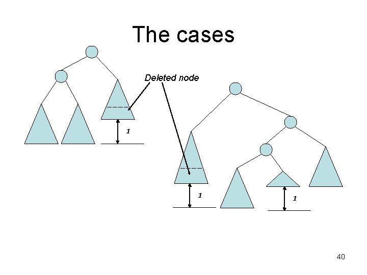
The same applies for deleting • Only 2 cases (an their mirrors) – The element is deleted at the right (left) subtree of which was already smaller than the left (right) sub-tree by 1 – The new element is inserted at the left (right) sub-tree of the right (left) child which was already higher that the left (right) sub-tree by 1 39

The cases Deleted node 1 1 1 40

Re-balancing after deleting: After deleting a node the tree might be still balanced or: Theorem: after deleting we can restore the AVL balance properties of the sub-tree having as root the first* node that got unbalanced with just only one simple rotation or a double rotation. (* : on the way from the deleted note to the root). However: the height of the resulting sub-tree might be shortened by 1, this means more rotations might be (recursively) necessary at the parent nodes, which can affect up to the root of the entire tree. 41

About Implementation § § § While searching for unbalanced sub-tree after an operation it is only necessary to check the parent´s sub-tree only when the son´s sub-tree has changed it height. In order make the checking for unbalanced sub-trees more efficient, it is recommended to put some more information on the nodes, for example: the height of the sub-tree or the balance factor (height(left sub-tree) – height(right sub-tree)) This information must be updated after each operation It is necessary to have an operation that returns the parent of a certain node (for example, by adding a pointer to the parent). 42

Complexity analysis– worst case Be h the height of the AVL-tree. Searching: as in the normal binary search tree O(h). Insert: the insertion is the same as the binary search tree (O(h)) but we must add the cost of one simple or double rotation, which is constant : also O(h). delete: delete as in the binary search tree(O(h)) but we must add the cost of (possibly) one rotation at each node on the way from the deleted node to the root, which is at most the height of the tree: O(h). All operations are O(h). 43

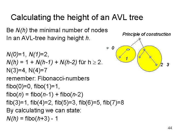
Calculating the height of an AVL tree Be N(h) the minimal number of nodes In an AVL-tree having height h. Principle of construction 0 N(0)=1, N(1)=2, 1 N(h) = 1 + N(h-1) + N(h-2) für h 2. N(3)=4, N(4)=7 remember: Fibonacci-numbers fibo(0)=0, fibo(1)=1, fibo(n) = fibo(n-1) + fibo(n-2) fib(3)=1, fib(4)=2, fib(5)=3, fib(6)=5, fib(7)=8 By calculating we can state: N(h) = fibo(h+3) - 1 2 3 44

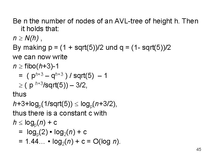
Be n the number of nodes of an AVL-tree of height h. Then it holds that: n N(h) , By making p = (1 + sqrt(5))/2 und q = (1 - sqrt(5))/2 we can now write n fibo(h+3)-1 = ( ph+3 – qh+3 ) / sqrt(5) – 1 ( p h+3/sqrt(5)) – 3/2, thus h+3+logp(1/sqrt(5)) logp(n+3/2), thus there is a constant c with h logp(n) + c = logp(2) • log 2(n) + c = 1. 44… • log 2(n) + c = O(log n). 45

6. 3. 1 Heapsort Idea: two phases: 1. Construction of the heap 2. Output of the heap For ordering number in an ascending sequence: use a Heap with reverse order: the maximum number should be at the root (not the minimum). Heapsort is an in-situ-Procedure 46

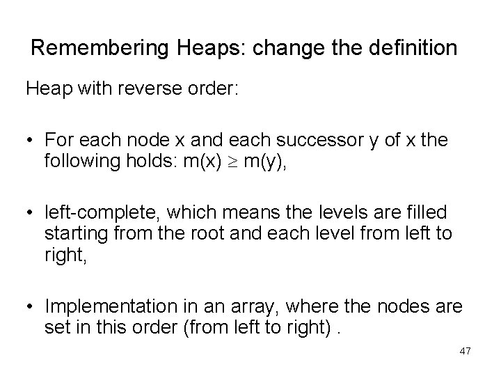
Remembering Heaps: change the definition Heap with reverse order: • For each node x and each successor y of x the following holds: m(x) m(y), • left-complete, which means the levels are filled starting from the root and each level from left to right, • Implementation in an array, where the nodes are set in this order (from left to right). 47

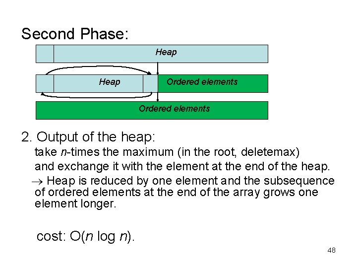
Second Phase: Heap Ordered elements Ordered elements 2. Output of the heap: take n-times the maximum (in the root, deletemax) and exchange it with the element at the end of the heap. Heap is reduced by one element and the subsequence of ordered elements at the end of the array grows one element longer. cost: O(n log n). 48

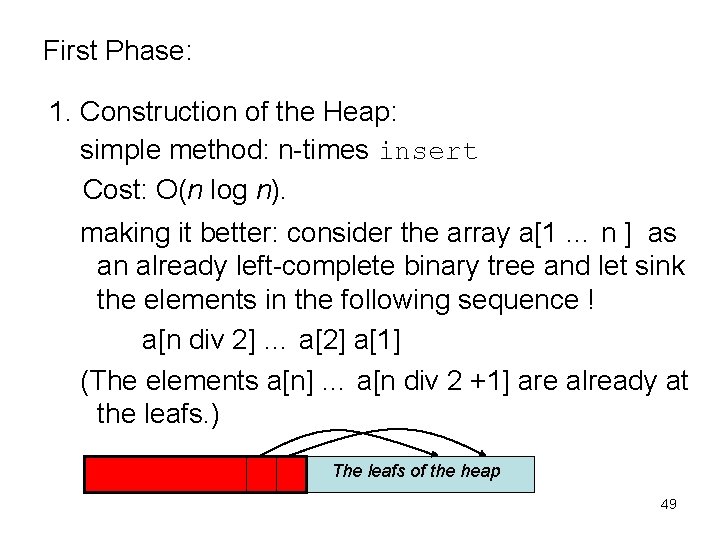
First Phase: 1. Construction of the Heap: simple method: n-times insert Cost: O(n log n). making it better: consider the array a[1 … n ] as an already left-complete binary tree and let sink the elements in the following sequence ! a[n div 2] … a[2] a[1] (The elements a[n] … a[n div 2 +1] are already at the leafs. ) HH The leafs of the heap 49

Formally: heap segment an array segment a[ i. . k ] ( 1 i k <=n ) is said to be a heap segment when following holds: for all j from {i, . . . , k} m(a[ j ]) m(a[ 2 j ]) if 2 j k and m(a[ j ]) m(a[ 2 j+1]) if 2 j+1 k If a[i+1. . n] is already a heap segment we can convert a[i…n] into a heap segment by letting a[i] sink. 50

Cost calculation Be k = [log n+1]+ - 1. (the height of the complete portion of the heap) cost: For an element at level j from the root: k – j. alltogether: {j=0, …, k} (k-j) • 2 j = 2 k • {i=0, …, k} i/2 i =2 • 2 k = O(n). 51

advantage: The new construction strategy is more efficient ! Usage: when only the m biggest elements are required: 1. construction in O(n) steps. 2. output of the m biggest elements in O(m • log n) steps. total cost: O( n + m • log n). 52

Addendum: Sorting with search trees Algorithm: 1. Construction of a search tree (e. g. AVL-tree) with the elements to be sorted by n insert opeartions. 2. Output of the elements in In. Order-sequence. Ordered sequence. cost: 1. O(n log n) with AVL-trees, 2. O(n). in total: O(n log n). optimal! 53