CHAPTER 6 REGRESSION DIAGNOSTIC III AUTOCORRELATION Damodar Gujarati

CHAPTER 6 REGRESSION DIAGNOSTIC III: AUTOCORRELATION Damodar Gujarati Econometrics by Example

AUTOCORRELATION Ø One of the assumptions of the classical linear regression (CLRM) is that the covariance between ui, the error term for observation i, and uj, the error term for observation j, is zero. Ø Reasons for autocorrelation include: Ø The possible strong correlation between the shock in time t with the shock in time t+1 Ø More common in time series data Damodar Gujarati Econometrics by Example

CONSEQUENCES Ø If autocorrelation exists, several consequences ensue: Ø The OLS estimators are still unbiased and consistent. Ø They are still normally distributed in large samples. Ø They are no longer efficient, meaning that they are no longer BLUE. Ø In most cases standard errors are underestimated. Ø Thus, the hypothesis-testing procedure becomes suspect, since the estimated standard errors may not be reliable, even asymptotically (i. e. , in large samples). Damodar Gujarati Econometrics by Example

DETECTION OF AUTOCORRELATION Ø Graphical method Ø Plot the values of the residuals, et, chronologically Ø If discernible pattern exists, autocorrelation likely a problem Ø Durbin-Watson test Ø Breusch-Godfrey (BG) test Damodar Gujarati Econometrics by Example

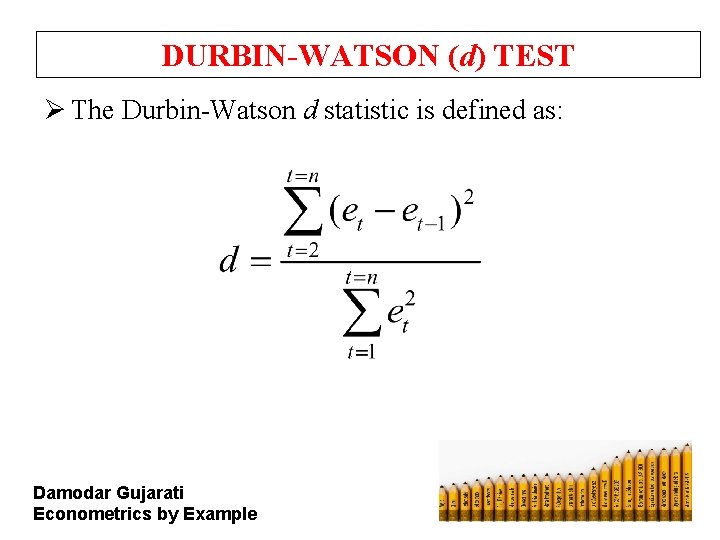
DURBIN-WATSON (d) TEST Ø The Durbin-Watson d statistic is defined as: Damodar Gujarati Econometrics by Example

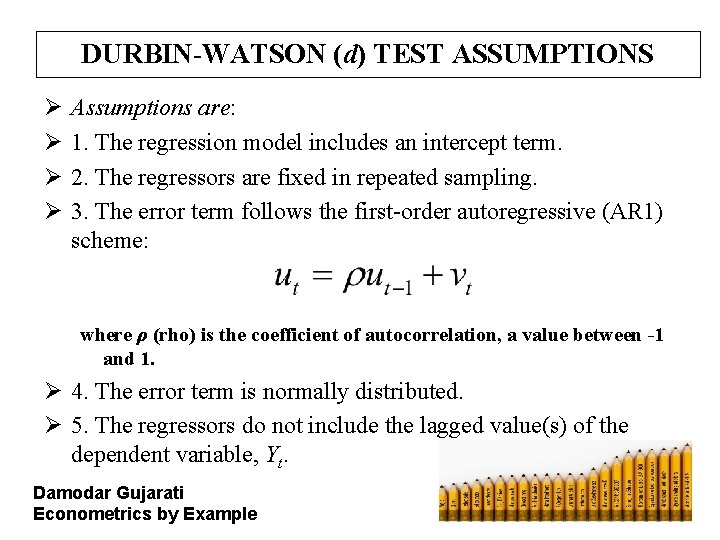
DURBIN-WATSON (d) TEST ASSUMPTIONS Ø Ø Assumptions are: 1. The regression model includes an intercept term. 2. The regressors are fixed in repeated sampling. 3. The error term follows the first-order autoregressive (AR 1) scheme: where ρ (rho) is the coefficient of autocorrelation, a value between -1 and 1. Ø 4. The error term is normally distributed. Ø 5. The regressors do not include the lagged value(s) of the dependent variable, Yt. Damodar Gujarati Econometrics by Example

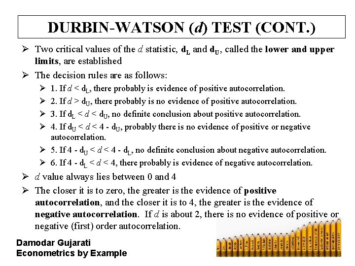
DURBIN-WATSON (d) TEST (CONT. ) Ø Two critical values of the d statistic, d. L and d. U, called the lower and upper limits, are established Ø The decision rules are as follows: Ø Ø 1. If d < d. L, there probably is evidence of positive autocorrelation. 2. If d > d. U, there probably is no evidence of positive autocorrelation. 3. If d. L < d. U, no definite conclusion about positive autocorrelation. 4. If d. U < d < 4 - d. U, probably there is no evidence of positive or negative autocorrelation. Ø 5. If 4 - d. U < d < 4 - d. L, no definite conclusion about negative autocorrelation. Ø 6. If 4 - d. L < d < 4, there probably is evidence of negative autocorrelation. Ø d value always lies between 0 and 4 Ø The closer it is to zero, the greater is the evidence of positive autocorrelation, and the closer it is to 4, the greater is the evidence of negative autocorrelation. If d is about 2, there is no evidence of positive or negative (first) order autocorrelation. Damodar Gujarati Econometrics by Example

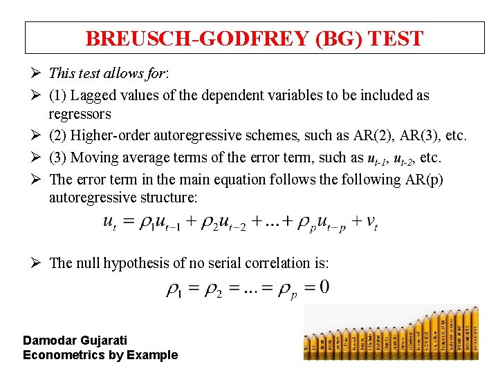
BREUSCH-GODFREY (BG) TEST Ø This test allows for: Ø (1) Lagged values of the dependent variables to be included as regressors Ø (2) Higher-order autoregressive schemes, such as AR(2), AR(3), etc. Ø (3) Moving average terms of the error term, such as ut-1, ut-2, etc. Ø The error term in the main equation follows the following AR(p) autoregressive structure: Ø The null hypothesis of no serial correlation is: Damodar Gujarati Econometrics by Example

BREUSCH-GODFREY (BG) TEST (CONT. ) Ø The BG test involves the following steps: Ø Regress et, the residuals from our main regression, on the regressors in the model and the p autoregressive terms given in the equation on the previous slide, and obtain R 2 from this auxiliary regression. Ø If the sample size is large, BG have shown that: (n – p)R 2 ~ X 2 p Ø That is, in large samples, (n – p) times R 2 follows the chi-square distribution with p degrees of freedom. Ø Rejection of the null hypothesis implies evidence of autocorrelation. Ø As an alternative, we can use the F value obtained from the auxiliary regression. Ø This F value has (p , n-k-p) degrees of freedom in the numerator and denominator, respectively, where k represents the number of parameters in the auxiliary regression (including the intercept term). Damodar Gujarati Econometrics by Example

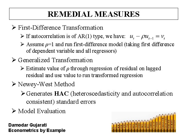
REMEDIAL MEASURES Ø First-Difference Transformation Ø If autocorrelation is of AR(1) type, we have: Ø Assume ρ=1 and run first-difference model (taking first difference of dependent variable and all regressors) Ø Generalized Transformation Ø Estimate value of ρ through regression of residual on lagged residual and use value to run transformed regression Ø Newey-West Method Ø Generates HAC (heteroscedasticity and autocorrelation consistent) standard errors Ø Model Evaluation Damodar Gujarati Econometrics by Example