Chapter 6 Production and Cost One Variable Input

Production Function u The production function identifies the maximum quantity of good y that can be produced from any input bundle (z 1, z 2). u A production function is stated as: y=F(z 1, z 2). 6/2 © 2009 Pearson Education Canada

Production Functions u In a fixed proportions production function, the ratio in which the inputs are used never varies. u In a variable proportion production function, the ratio of inputs can vary. 6/3 © 2009 Pearson Education Canada

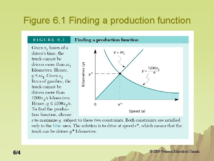
Figure 6. 1 Finding a production function 6/4 © 2009 Pearson Education Canada

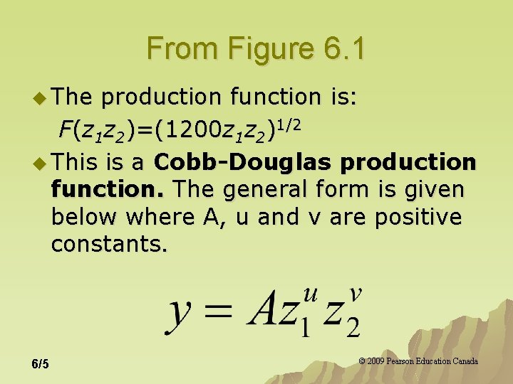
From Figure 6. 1 u The production function is: F(z 1 z 2)=(1200 z 1 z 2)1/2 u This is a Cobb-Douglas production function. The general form is given below where A, u and v are positive constants. 6/5 © 2009 Pearson Education Canada

Costs u Opportunity cost is the value of the highest forsaken alternative. u Sunk costs are costs that, once incurred, cannot be recovered. u Avoidable costs are costs that need not be incurred (can be avoided). u Fixed costs do not vary with output. u Variable costs change with output. 6/6 © 2009 Pearson Education Canada

Long-Run Cost Minimization u u 1. 2. 6/7 The goal is to choose quantities of inputs z 1 and z 2 that minimize total costs, subject to being able to produce y units of output. That is: Minimize w 1 z 1+w 2 z 2 (w 1, w 2 are input prices). Choosing z 1 and z 2 subject to the constraint y=F(z 1, z 2). © 2009 Pearson Education Canada

Production: One Variable Input u Total production function TP (z 1) (z 2 fixed at 105) defined as: TP (z 1)=F(z 1, 105) u Marginal product MP(z 1) is the rate of output change when the variable input changes (given fixed amounts of all other inputs). u MP (z 1)=slope of TP (z 1) 6/8 © 2009 Pearson Education Canada

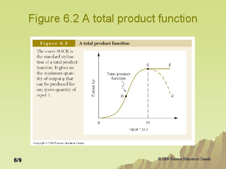
Figure 6. 2 A total product function 6/9 © 2009 Pearson Education Canada

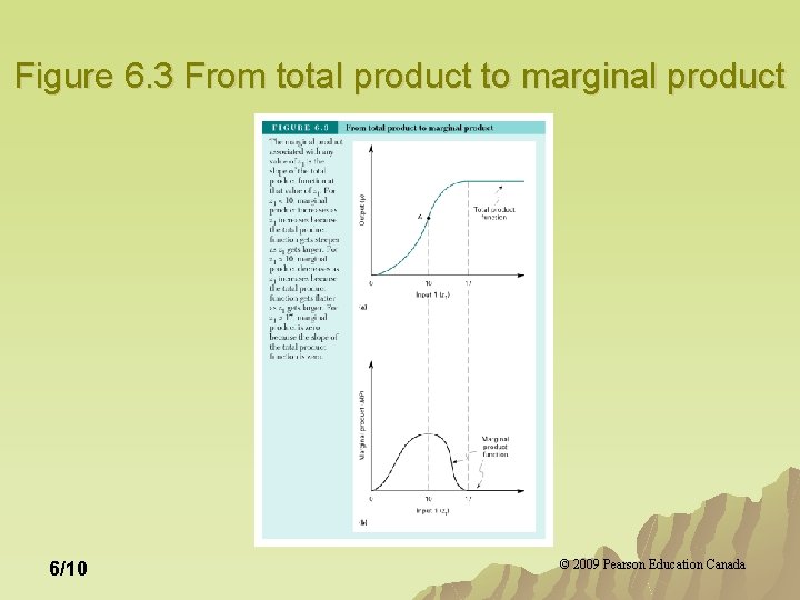
Figure 6. 3 From total product to marginal product 6/10 © 2009 Pearson Education

The Free-disposal Assumption Because a production function gives the maximum output from any input combination, we assume that increased amounts of inputs will not be used if they negatively impact output. u This is sometimes called the freedisposal assumption and combined with our definition of the production function, implies that marginal product cannot be negative. u 6/11 © 2009 Pearson Education Canada

The Free-disposal Assumption u Given the free-disposal assumption, the marginal product of any input is always greater than or equal to zero. u Furthermore, for any input bundle, the marginal product of at least one input is positive. 6/12 © 2009 Pearson Education Canada

Diminishing Marginal Productivity Reflects the assumption that at some point the rate of increase in total output (marginal product) will begin to decline. u Suppose the quantities of all inputs except one - say, input 1 - are fixed. There is a quantity of input 1 - say, z” 1 - such that whenever z 1 exceeds z” 1, the marginal product of input 1 decreases as z 1 increases. u 6/13 © 2009 Pearson Education Canada

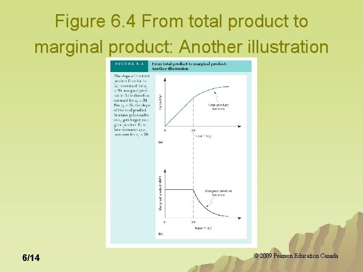
Figure 6. 4 From total product to marginal product: Another illustration 6/14 © 2009

Average Product u Average product (AP) of the variable input equals total output divided

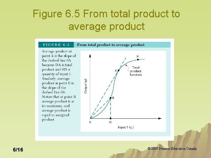
Figure 6. 5 From total product to average product 6/16 © 2009 Pearson Education

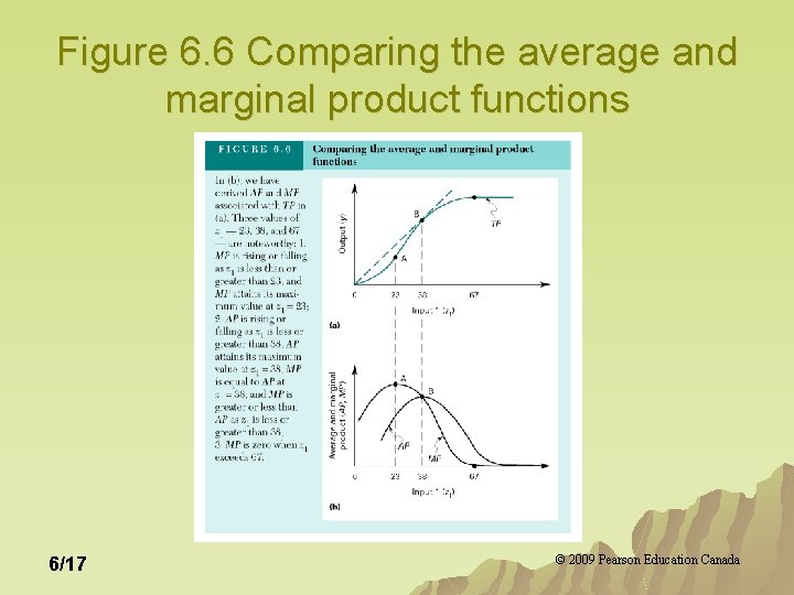
Figure 6. 6 Comparing the average and marginal product functions 6/17 © 2009 Pearson

Marginal and Average Product 1. 2. 3. When 6/18 MP exceeds AP, AP is

Costs of Production: One Variable Input u The cost-minimization problem is: Minimize w 1 z 1 by choice of z 1. Subject to constraint y=TP(z 1). u The variable cost function, VC(y) is: VC(y)=the minimum variable cost of producing y units of output. 6/19 © 2009 Pearson Education Canada

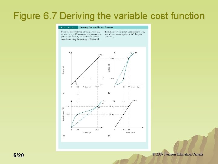
Figure 6. 7 Deriving the variable cost function 6/20 © 2009 Pearson Education Canada

More Costs u Average variable cost is variable cost per unit of output. AV(y)=VC(y)/y u Short-run marginal cost is the rate at which costs increase in the shortrun. SMC(y)=slope of VC(y) 6/21 © 2009 Pearson Education Canada

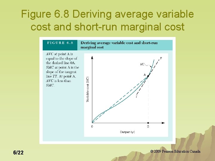
Figure 6. 8 Deriving average variable cost and short-run marginal cost 6/22 © 2009

Short-run Marginal Costs and Average Variable Costs 1. 2. 3. 6/23 When SMC is below AVC, AVC decreases as y increases. When SMC is equal to AVC, AVC is constant (its slope is zero). When SMC is above AVC, AVC increases as y increases. © 2009 Pearson Education Canada

Average Product and Average Cost AVC (y’)=w 1/AP(z 1’) u The average variable cost

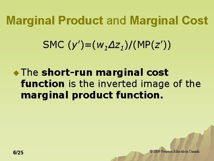
Marginal Product and Marginal Cost SMC (y’)=(w 1Δz 1)/(MP(z’)) u The short-run marginal cost

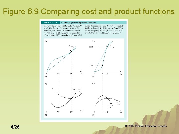
Figure 6. 9 Comparing cost and product functions 6/26 © 2009 Pearson Education Canada

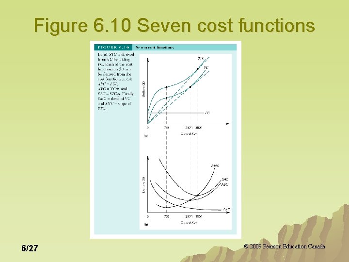
Figure 6. 10 Seven cost functions 6/27 © 2009 Pearson Education Canada

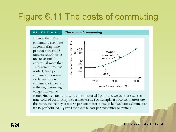
Figure 6. 11 The costs of commuting 6/28 © 2009 Pearson Education Canada

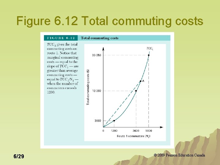
Figure 6. 12 Total commuting costs 6/29 © 2009 Pearson Education Canada

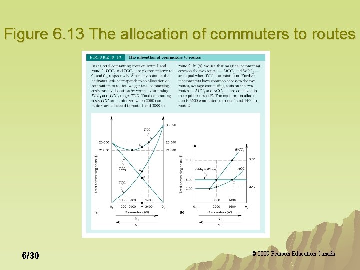
Figure 6. 13 The allocation of commuters to routes 6/30 © 2009 Pearson Education

Application: The Allocation of Output Among Different Plants u Let us reinterpret the lessons from traffic congestion to solve a problem related to multi-plant firms. u The firm’s problem is to allocate output to its two plants so as to minimize its total variable cost. 6/31 © 2009 Pearson Education Canada

Application: The Allocation of Output Among Different Plants u Think of Figure 6. 13 as the variable and marginal cost functions associated with two plants (TCC 1, TCC 2 and MC 1, MC 2) respectively. u The curve TCC in Figure 6. 13 a tells us that the firm can minimize the variable costs of producing 5000 units by allocating 2000 units to the first plant and 3000 units to the second plant. 6/32 © 2009 Pearson Education Canada

Application: The Allocation of Output Among Different Plants u Using the logic from Figure 6. 13 b: – Total costs can be reduced by allocating output from the high-marginal cost plant to the low-cost marginal plant. – To minimize the total variable cost of producing a given output in two or more plants, a firm allocates output to the plants so that short-run marginal cost is the same in all plants. 6/33 © 2009 Pearson Education Canada