Chapter 6 Probability and Simulation 6 1 Simulation

Chapter 6 Probability and Simulation 6. 1 Simulation

Simulation • The imitation of chance behavior based on a model that accurately reflects the experiment under consideration, is called a simulation

Steps for Conducting a Simulation 1. State the problem or describe the experiment 2. State the assumptions 3. Assign digits to represent outcomes 4. Simulate many repetitions 5. State your conclusions

Step 1: State the problem or describe the experiment • Toss a coin 10 times. What is the likelihood of a run of at least 3 consecutive heads or 3 consecutive tails?

Step 2: State the Assumptions • There are Two – A head or tail is equally likely to occur on each toss – Tosses are independent of each other (ie: what happens on one toss will not influence the next toss).

Step 3 Assign Digits to represent outcomes • Since each outcome is just as likely as the other, and there you are just as likely to get an even number as an odd number in a random number table or using a random number generator, assign heads odds and tails evens.

Step 4 Simulate many repetitions • Looking at 10 consecutive digits in Table B (or generating 10 random numbers) simulates one repetition. Read many groups of 10 digits from the table to simulate many repetitions. Keep track of whether or not the event we want ( a run of 3 heads or 3 tails) occurs on each repetition. Example 6. 3 on page 394

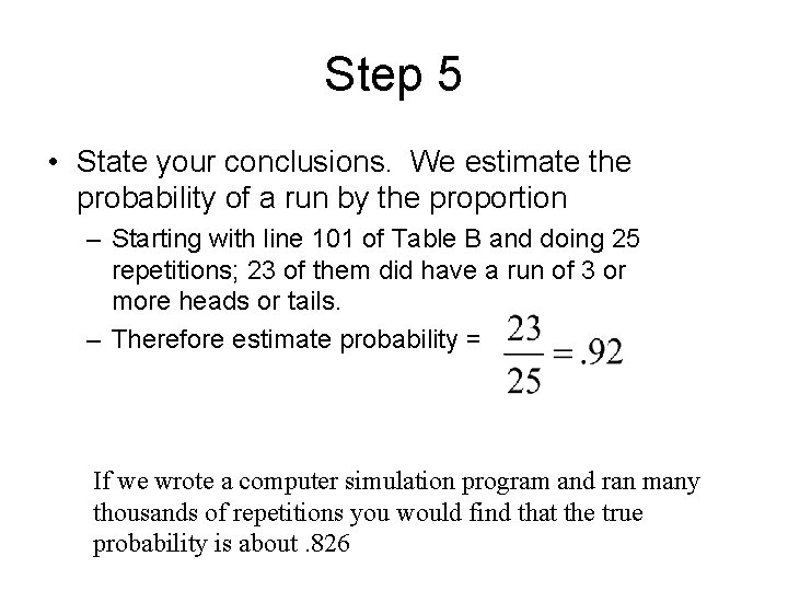
Step 5 • State your conclusions. We estimate the probability of a run by the proportion – Starting with line 101 of Table B and doing 25 repetitions; 23 of them did have a run of 3 or more heads or tails. – Therefore estimate probability = If we wrote a computer simulation program and ran many thousands of repetitions you would find that the true probability is about. 826

Various Simulation Scenarios • Example 6. 4 – page 395 - Choose one person at random from a group of 70% employed. Simulate using random number table.

Frozen Yogurt Sales • Example 6. 5 – page 396 – Using random number table simulate the flavor choice of 10 customers entering shop given historic sales of 38% chocolate, 42% vanilla, 20% strawberry.

A Girl or Four • Example 6. 6 – Page 396 – Use Random number table to simulate a couple have children until 1 is a girl or have four children. Perform 14 Simulation

Simulation with Calculator • Activity 6 B – page 399 – Simulate the random firing of 10 Salespeople where 24% of the sales force are age 55 or above. (20 repetitions)

Homework • Read 6. 1, 6. 2 • Complete Problems 1 -4, 8, 9, 12

Chapter 6 Probability and Simulation 6. 2 Probability Models

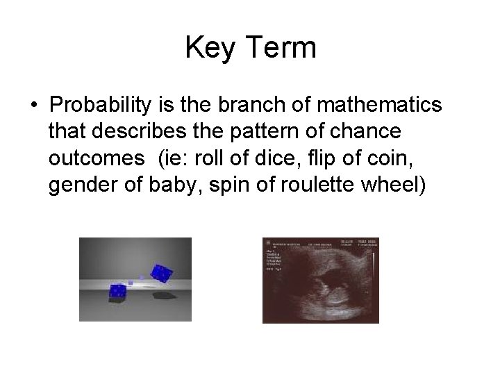
Key Term • Probability is the branch of mathematics that describes the pattern of chance outcomes (ie: roll of dice, flip of coin, gender of baby, spin of roulette wheel)

Key Concept • “Random” in statistics is not a synonym of “haphazard” but a description of a kind of order that emerges only in the long run

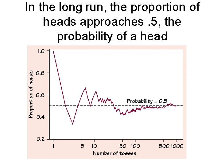
In the long run, the proportion of heads approaches. 5, the probability of a head

Researchers with Time on their Hands • French Naturalist Count Buffon (1707 – 1788) tossed a coin 4040 time. Results: 2048 head or a proportion of. 5069. • English Statistictian Karl Person 24, 000 times. Results 12, 012, a proportion of. 5005. • Austrailian mathematician and WWII POW John Kerrich tossed a coin 10, 000 times. Results 5067 heads, proportion of heads. 5067

Key Term / Concept • We call a phenomenon random if individual outcomes are uncertain but there is nonetheless a regular distribution of outcomes in a large number of repetitions

Key Term / Concept • The probability of any outcome of a random phenomenon is the proportion of times the outcome would occur in a very long series of repetition.

Key Term / Concept As you explore randomness, remember – You must have a long series of independent trials. (The outcome of one trial must not influence the outcome of any other trial) – We can estimate a real-world probability only by observing many trials. – Computer Simulations are very useful because we need long runs of data.

Key Term / Concept The sample space S of a random phenomenon is the set of all possible outcomes. Example: The sample space for a toss of a coin. S = {heads, tails}

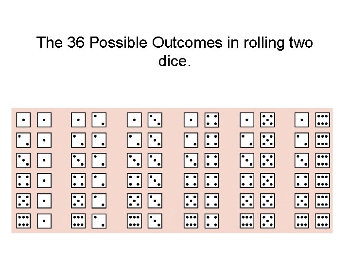
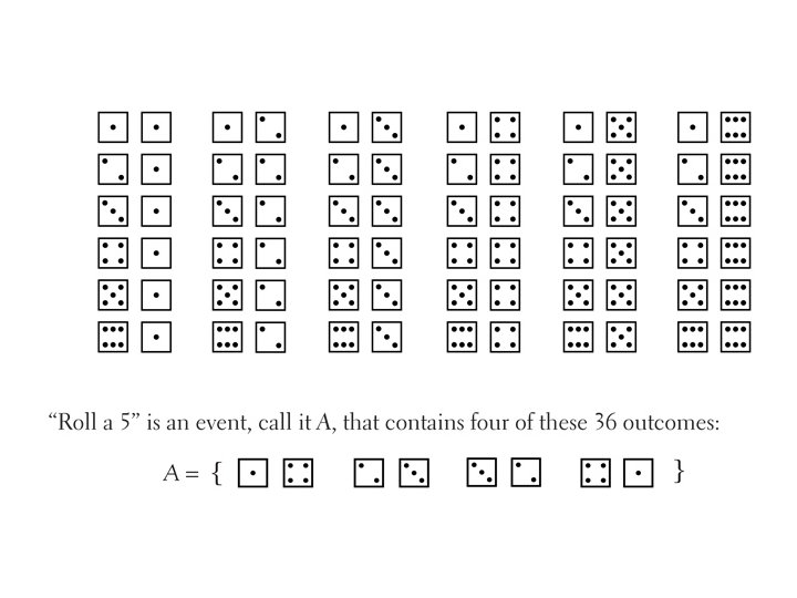
The 36 Possible Outcomes in rolling two dice.

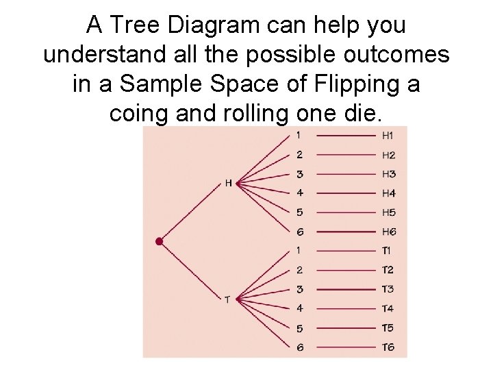
A Tree Diagram can help you understand all the possible outcomes in a Sample Space of Flipping a coing and rolling one die.

Key Concept Multiplication Principle - If you can do one task in n 1 number of ways and a second task in n 2 number of ways, then both tasks can be done in n 1 x n 2 number of ways. ie: flipping a coin and rolling a die, 2 x 6 = 12 different possible outcomes

Key Term / Concept • With Replacement – Draw a ball out of bag. Observe the ball. Then return ball to bag. • Without Replacement – Draw a ball out of bag. Observe the ball. The ball is not returned to bag.

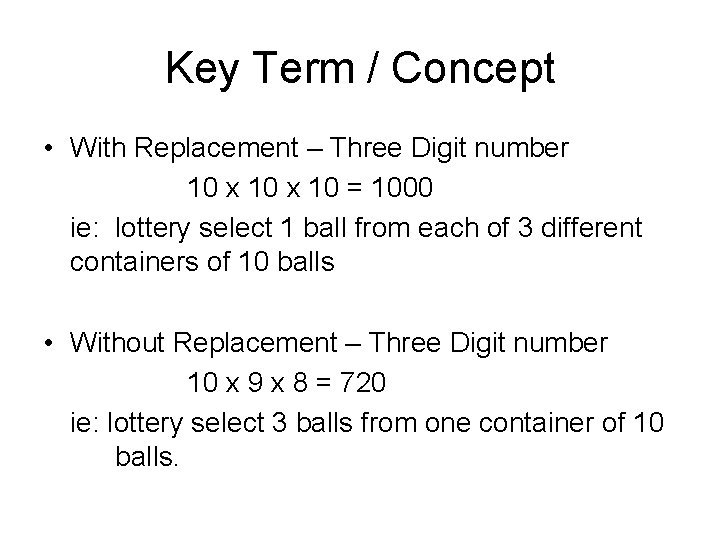
Key Term / Concept • With Replacement – Three Digit number 10 x 10 = 1000 ie: lottery select 1 ball from each of 3 different containers of 10 balls • Without Replacement – Three Digit number 10 x 9 x 8 = 720 ie: lottery select 3 balls from one container of 10 balls.

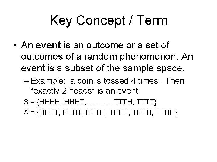
Key Concept / Term • An event is an outcome or a set of outcomes of a random phenomenon. An event is a subset of the sample space. – Example: a coin is tossed 4 times. Then “exactly 2 heads” is an event. S = {HHHH, HHHT, ………. . , TTTH, TTTT} A = {HHTT, HTHT, HTTH, THHT, THTH, TTHH}

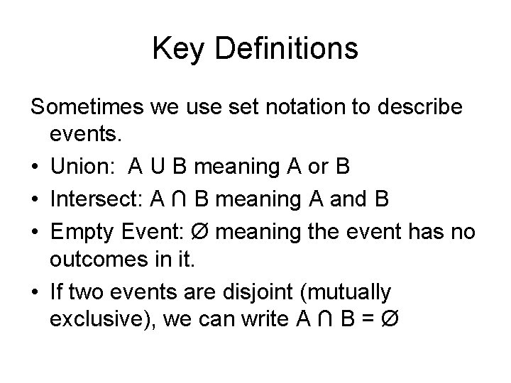
Key Definitions Sometimes we use set notation to describe events. • Union: A U B meaning A or B • Intersect: A ∩ B meaning A and B • Empty Event: Ø meaning the event has no outcomes in it. • If two events are disjoint (mutually exclusive), we can write A ∩ B = Ø

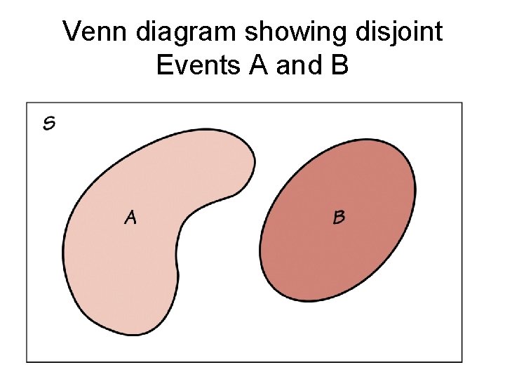
Venn diagram showing disjoint Events A and B

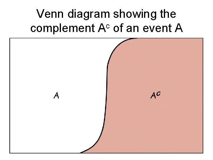
Venn diagram showing the complement Ac of an event A

Complement Example 6. 13 on page 419

Probabilities in a Finite Sample Space • Assign a Probability to each individual outcome. The probabilities must be numbers between 0 and 1 and must have a sum 1. • The probability of any event is the sum of the outcomes making up the event Example 6. 14 page 420

Assigning Probabilities: equally likely outcomes • If a random phenomenon has k possible outcomes, all equally likely, then each individual outcome has probability 1/k. The probability of any event A is P(A) = count of outcomes in A count of outcomes in S Example: Dice, random digits…etc

The Multiplication Rule for Independent Events Rule 3. Two events A and B are independent if knowing that one occurs does not change the probability that the other occurs. If A and B are independent. P(A and B) = P(A)P(B) Examples: 6. 17 page 426

Homework • Read Section 6. 3 • Exercises 22, 24, 28, 29, 32 -33, 36, 38, 44

Probability And Simulation: The Study of Randomness 6. 3 General Probability Rules

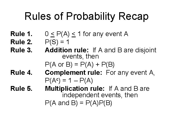
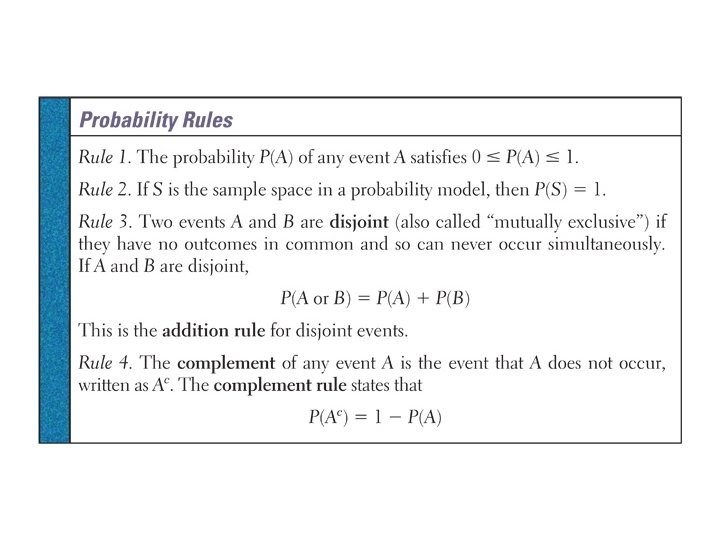
Rules of Probability Recap Rule 1. Rule 2. Rule 3. Rule 4. Rule 5. 0 < P(A) < 1 for any event A P(S) = 1 Addition rule: If A and B are disjoint events, then P(A or B) = P(A) + P(B) Complement rule: For any event A, P(Ac) = 1 – P(A) Multiplication rule: If A and B are independent events, then P(A and B) = P(A)P(B)

Key Term • The union of any collection of events is the event that at least one of the collection occurs.

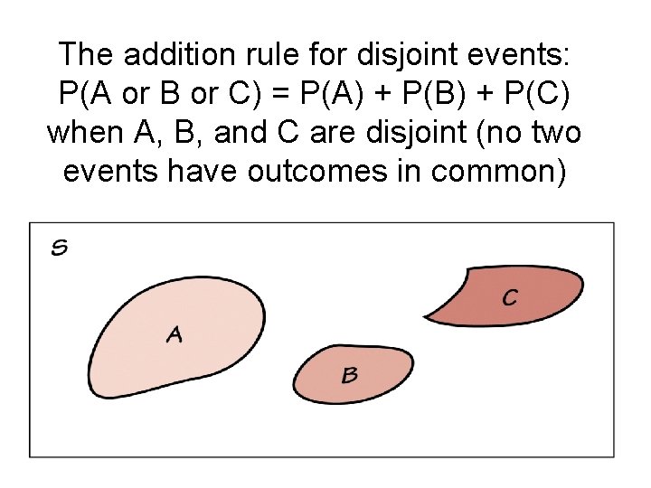
The addition rule for disjoint events: P(A or B or C) = P(A) + P(B) + P(C) when A, B, and C are disjoint (no two events have outcomes in common)

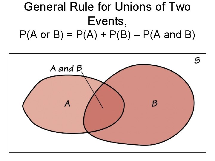
General Rule for Unions of Two Events, P(A or B) = P(A) + P(B) – P(A and B)

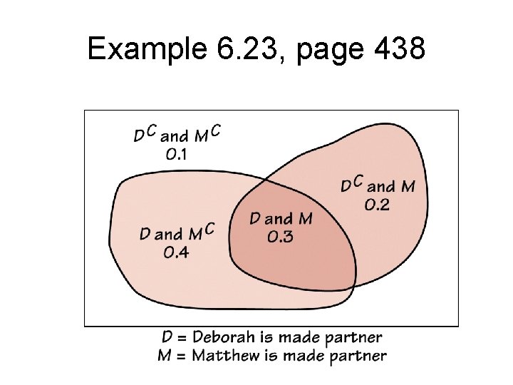
Example 6. 23, page 438

Conditional Probability • Example 6. 25, page 442, 443

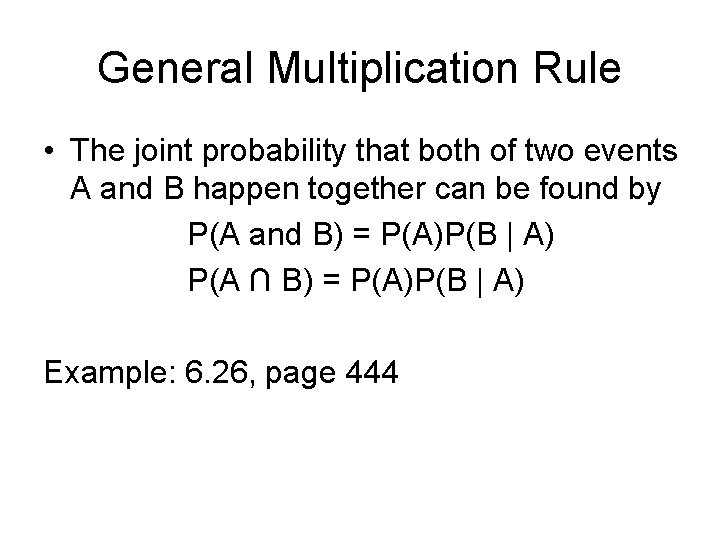
General Multiplication Rule • The joint probability that both of two events A and B happen together can be found by P(A and B) = P(A)P(B | A) P(A ∩ B) = P(A)P(B | A) Example: 6. 26, page 444

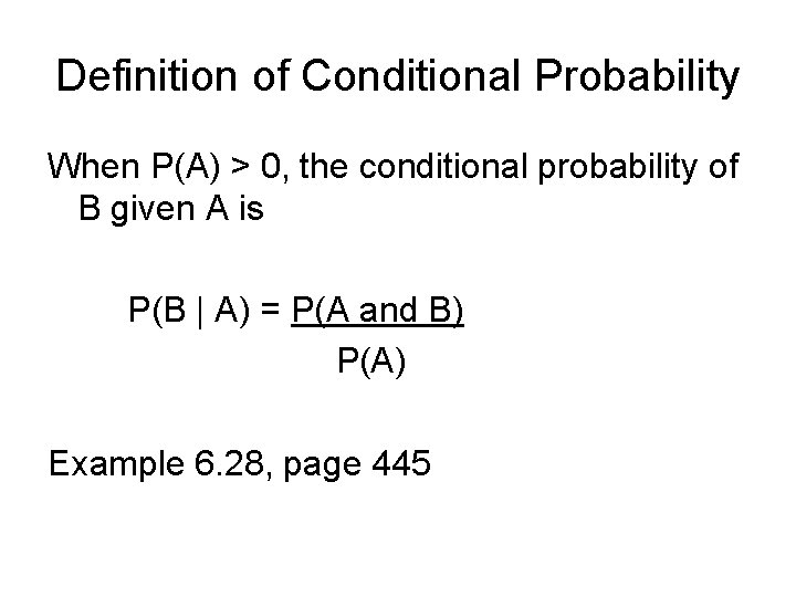
Definition of Conditional Probability When P(A) > 0, the conditional probability of B given A is P(B | A) = P(A and B) P(A) Example 6. 28, page 445

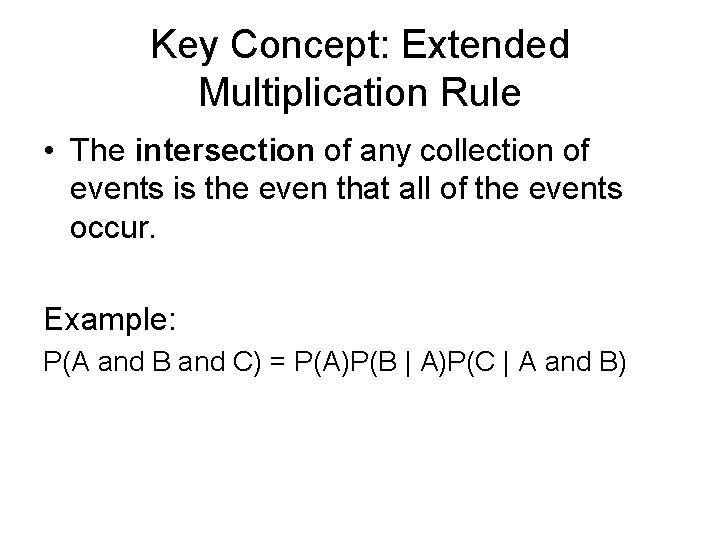
Key Concept: Extended Multiplication Rule • The intersection of any collection of events is the even that all of the events occur. Example: P(A and B and C) = P(A)P(B | A)P(C | A and B)

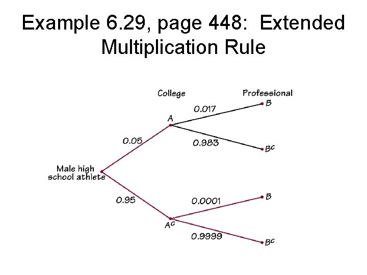
Example 6. 29, page 448: Extended Multiplication Rule

Tree Diagrams Revisted • Example 6. 30, Page 448 -9, Online Chatrooms

Bayes’s Rule • Example 6. 31, page 450, Chat Room Participants

Independence Again Two events A and B that both have positive probability are independent if P(B | A ) = P(B)

Homework • Exercises #71 -78, 82, 86 -88