Chapter 6 Part B Surface analysis gridding and

Chapter 6 Part B: Surface analysis – gridding and interpolation www. spatialanalysisonline. com

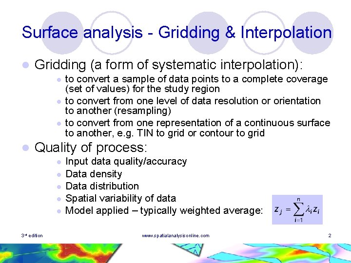
Surface analysis - Gridding & Interpolation l Gridding (a form of systematic interpolation): l l to convert a sample of data points to a complete coverage (set of values) for the study region to convert from one level of data resolution or orientation to another (resampling) to convert from one representation of a continuous surface to another, e. g. TIN to grid or contour to grid Quality of process: l l l 3 rd edition Input data quality/accuracy Data density Data distribution Spatial variability of data Model applied – typically weighted average: www. spatialanalysisonline. com 2

Surface analysis - Gridding & Interpolation l Some other key issues: ¡ Validity of continuity assumption/handling of breaklines/stratifications and missing data ¡ Validity of weighted average model ¡ How to choose weights? ¡ How many points to include in summation? ¡ Shape and size of neighbourhood region ¡ Selection of model and parameters ¡ Evaluation of quality ¡ Availability of related datasets 3 rd edition www. spatialanalysisonline. com 3

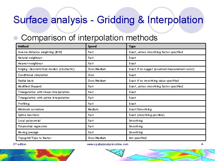
Surface analysis - Gridding & Interpolation l Comparison of interpolation methods Method Speed Type Inverse distance weighting (IDW) Fast Exact, unless smoothing factor specified Natural neighbour Fast Exact Nearest-neighbour Fast Exact Kriging -Geostatistical models (stochastic) Slow/Medium Exact if no nugget (assumed measurement error) Conditional simulation Slow Exact Radial basis Slow/Medium Exact if no smoothing value specified Modified Shepard Fast Exact, unless smoothing factor specified Triangulation with linear interpolation Fast Exact Triangulation with spline interpolation Fast Exact Profiling Fast Exact Minimum curvature Medium Exact/Smoothing Spline functions Fast Exact (smoothing possible) Local polynomial Fast Smoothing Polynomial regression Fast Smoothing Moving average Fast Smoothing Topogrid/Topo to Raster Slow/Medium Not specified 3 rd edition www. spatialanalysisonline. com 4

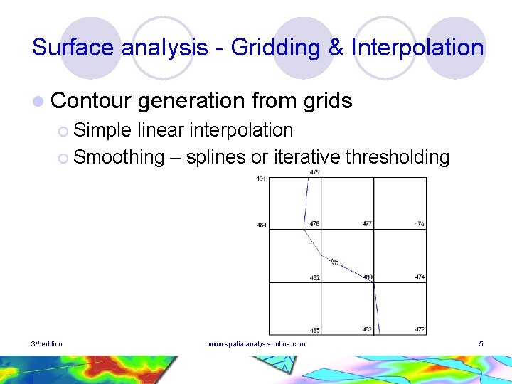
Surface analysis - Gridding & Interpolation l Contour generation from grids ¡ Simple linear interpolation ¡ Smoothing – splines or iterative thresholding 3 rd edition www. spatialanalysisonline. com 5

Surface analysis - Gridding & Interpolation Deterministic interpolation 3 rd edition www. spatialanalysisonline. com 6

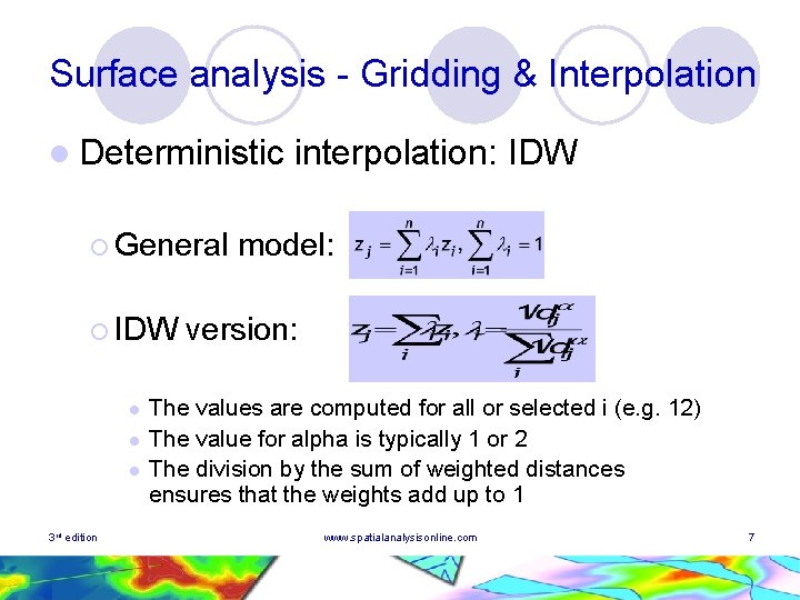
Surface analysis - Gridding & Interpolation l Deterministic ¡ General ¡ IDW l l l 3 rd edition interpolation: IDW model: version: The values are computed for all or selected i (e. g. 12) The value for alpha is typically 1 or 2 The division by the sum of weighted distances ensures that the weights add up to 1 www. spatialanalysisonline. com 7

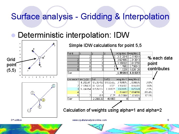
Surface analysis - Gridding & Interpolation l Deterministic interpolation: IDW Simple IDW calculations for point 5, 5 % each data point contributes Grid point (5, 5) Calculation of weights using alpha=1 and alpha=2 3 rd edition www. spatialanalysisonline. com 8

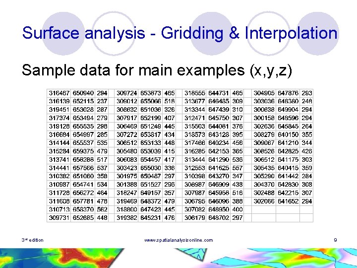
Surface analysis - Gridding & Interpolation Sample data for main examples (x, y, z) 3 rd edition www. spatialanalysisonline. com 9

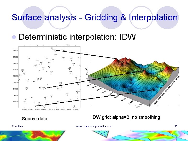
Surface analysis - Gridding & Interpolation l Deterministic Source data 3 rd edition interpolation: IDW grid: alpha=2, no smoothing www. spatialanalysisonline. com 10

Surface analysis - Gridding & Interpolation l IDW: ¡ ¡ ¡ All grid points in rectangle are assigned a value Sample points are exactly fitted Surface looks rather peaky with odd ‘hollows’/bull’s eye’s affected by point locations, alpha and grid resolution How do we know what values to choose - number of neighbours, alpha, grid res. , break lines? Can we judge the ‘goodness of fit’ of the resultant surface? l 3 rd edition Generally no, but could test the fit by (a) additional sampling; (b) comparison with other sources of data (e. g. aerial photographs); (c) computational procedures www. spatialanalysisonline. com 11

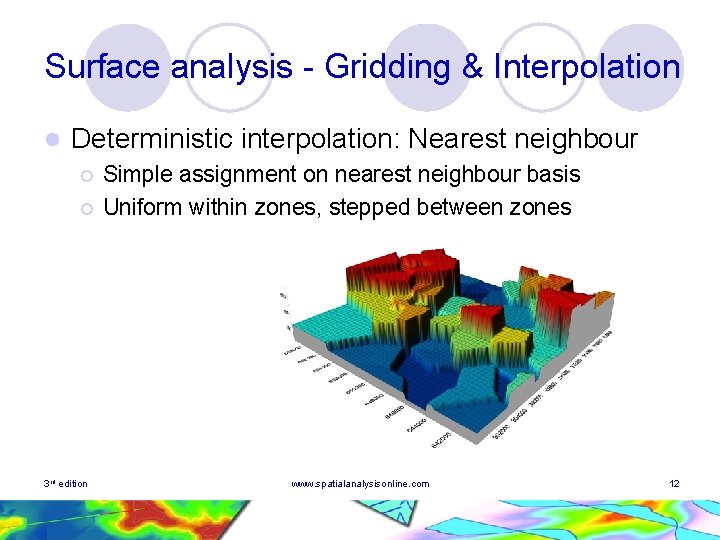
Surface analysis - Gridding & Interpolation l Deterministic interpolation: Nearest neighbour ¡ ¡ 3 rd edition Simple assignment on nearest neighbour basis Uniform within zones, stepped between zones www. spatialanalysisonline. com 12

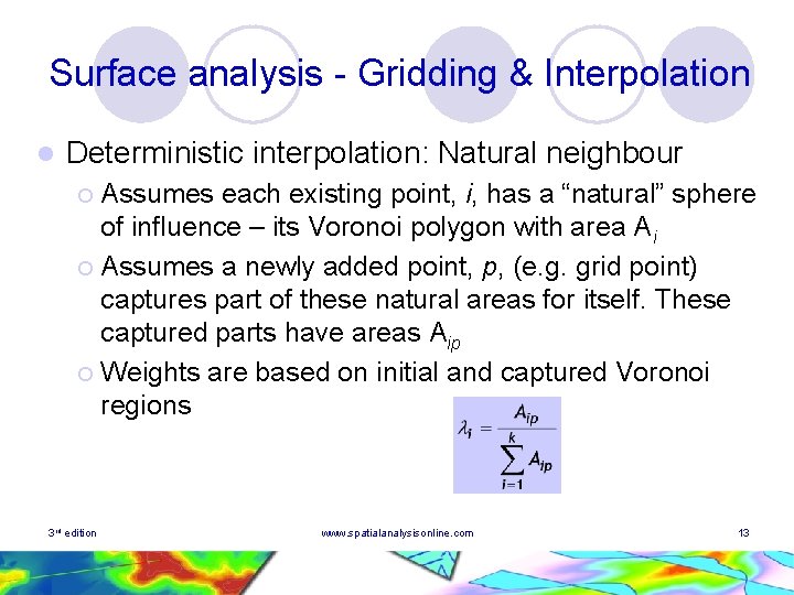
Surface analysis - Gridding & Interpolation l Deterministic interpolation: Natural neighbour Assumes each existing point, i, has a “natural” sphere of influence – its Voronoi polygon with area Ai ¡ Assumes a newly added point, p, (e. g. grid point) captures part of these natural areas for itself. These captured parts have areas Aip ¡ Weights are based on initial and captured Voronoi regions ¡ 3 rd edition www. spatialanalysisonline. com 13

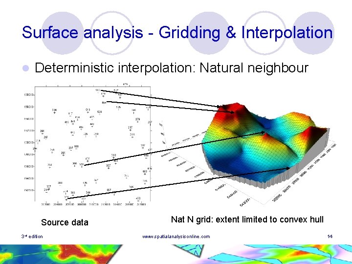
Surface analysis - Gridding & Interpolation l Deterministic interpolation: Natural neighbour Source data 3 rd edition Nat N grid: extent limited to convex hull www. spatialanalysisonline. com 14

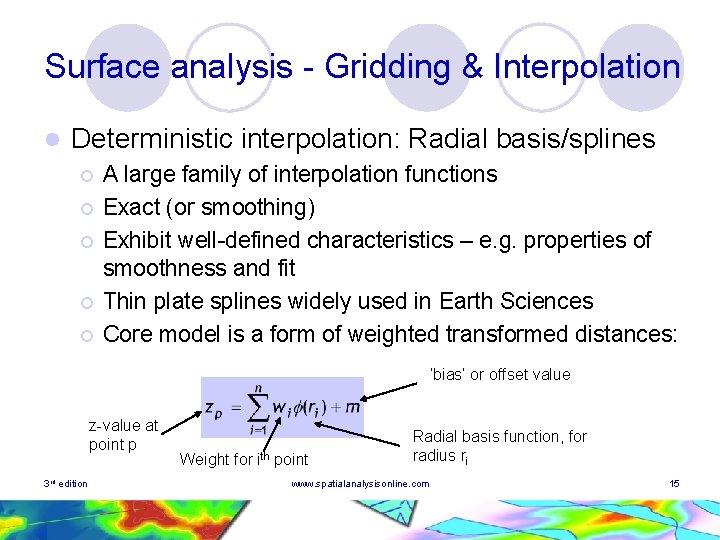
Surface analysis - Gridding & Interpolation l Deterministic interpolation: Radial basis/splines ¡ ¡ ¡ A large family of interpolation functions Exact (or smoothing) Exhibit well-defined characteristics – e. g. properties of smoothness and fit Thin plate splines widely used in Earth Sciences Core model is a form of weighted transformed distances: ‘bias’ or offset value z-value at point p 3 rd edition Weight for ith point Radial basis function, for radius ri www. spatialanalysisonline. com 15

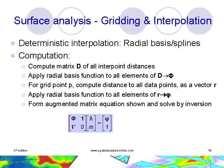
Surface analysis - Gridding & Interpolation Deterministic interpolation: Radial basis/splines l Computation: l ¡ ¡ ¡ 3 rd edition Compute matrix D of all interpoint distances Apply radial basis function to all elements of D For grid point p, compute distance to all data points, as a vector r Apply radial basis function to all elements of r Form augmented matrix equation shown and solve by inversion www. spatialanalysisonline. com 16

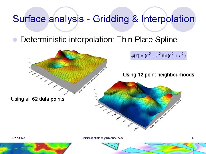
Surface analysis - Gridding & Interpolation l Deterministic interpolation: Thin Plate Spline Using 12 point neighbourhoods Using all 62 data points 3 rd edition www. spatialanalysisonline. com 17

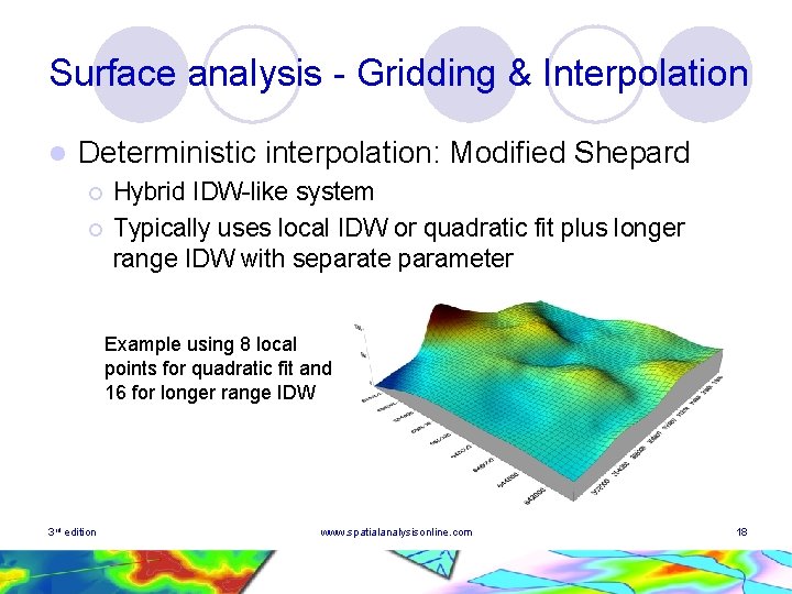
Surface analysis - Gridding & Interpolation l Deterministic interpolation: Modified Shepard ¡ ¡ Hybrid IDW-like system Typically uses local IDW or quadratic fit plus longer range IDW with separate parameter Example using 8 local points for quadratic fit and 16 for longer range IDW 3 rd edition www. spatialanalysisonline. com 18

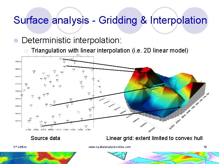
Surface analysis - Gridding & Interpolation l Deterministic interpolation: ¡ Triangulation with linear interpolation (i. e. 2 D linear model) Source data 3 rd edition Linear grid: extent limited to convex hull www. spatialanalysisonline. com 19

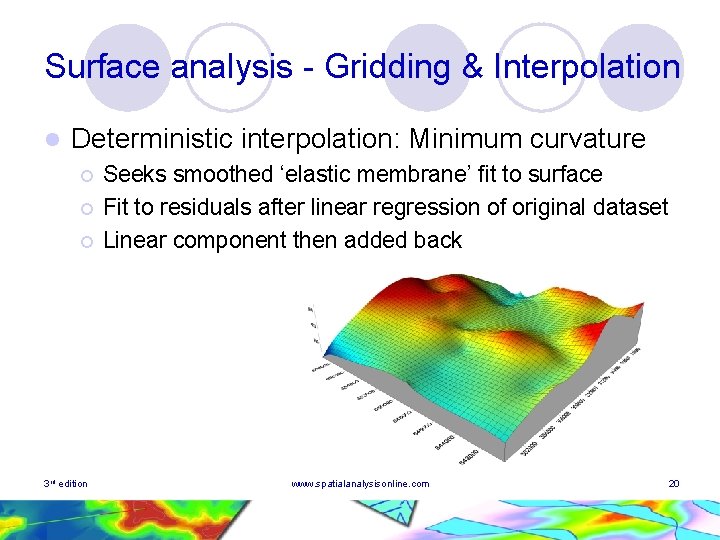
Surface analysis - Gridding & Interpolation l Deterministic interpolation: Minimum curvature ¡ ¡ ¡ 3 rd edition Seeks smoothed ‘elastic membrane’ fit to surface Fit to residuals after linear regression of original dataset Linear component then added back www. spatialanalysisonline. com 20

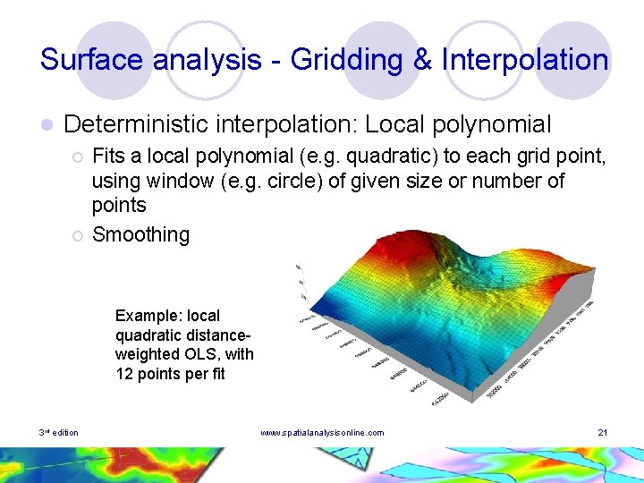
Surface analysis - Gridding & Interpolation l Deterministic interpolation: Local polynomial ¡ ¡ Fits a local polynomial (e. g. quadratic) to each grid point, using window (e. g. circle) of given size or number of points Smoothing Example: local quadratic distanceweighted OLS, with 12 points per fit 3 rd edition www. spatialanalysisonline. com 21

Surface analysis - Gridding & Interpolation l Deterministic interpolation – some other methods: ¡ ¡ ¡ 3 rd edition Triangulation with non-linear interpolation - Clough-Tocher: bicubic patches fitted to every triangle, such that edge and vertex joins are smooth Bi-linear: suitable for dense uniform datasets, e. g. grids with some missing cell values – simple weighted averaging of directly or indirectly neighbouring cells/points Profiling: input dataset is contour vectors. Typically interpolation is linear between closest pair of contours (8 -point) Moving average – uses a moving circular or elliptical window (similar to time series analysis) to obtain simple local average Topogrid – conversion of contour vectors to hydrologically consistent DEM. Includes enforcement of local drainage, lake boundaries, ridges and stream lines www. spatialanalysisonline. com 22

Surface analysis - Gridding & Interpolation Geostatistical interpolation 3 rd edition www. spatialanalysisonline. com 23

Surface analysis - Gridding & Interpolation l Geostatistical interpolation: Core concepts Geostatistics definition: “…models and methods for data observed at a discrete set of locations, such that the observed value, zi, is either a direct measurement of, or is statistically related to, the value of an underlying continuous spatial phenomenon, F(x, y), at the corresponding sampled location (xi, yi) within some spatial region A. ” (Diggle et al) 3 rd edition www. spatialanalysisonline. com 24

Surface analysis - Gridding & Interpolation l Geostatistical ¡ Addresses interpolation: Core concepts questions such as: how many points are needed to compute the local average? l what size, orientation and shape of neighbourhood should be chosen? l what model and weights should be used to compute the local average? l what errors (uncertainties) are associated with interpolated values? l 3 rd edition www. spatialanalysisonline. com 25

Surface analysis - Gridding & Interpolation l Geostatistical interpolation: Variograms ¡ Analyse the observed variation in data values by distance bands using a spatial autocorrelationlike measure, ¡ Typically, analyse all pairs of observations that lie within specific distance bands the average values of for each band ¡ Plot these averages against distance ¡ Fit an experimental curve to the observed pattern ¡ Compute 3 rd edition www. spatialanalysisonline. com 26

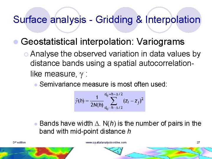
Surface analysis - Gridding & Interpolation l Geostatistical interpolation: Variograms ¡ Analyse the observed variation in data values by distance bands using a spatial autocorrelationlike measure, : l l 3 rd edition Semivariance measure is most often used: Bands have width . N(h) is the number of pairs in the band with mid-point distance h www. spatialanalysisonline. com 27

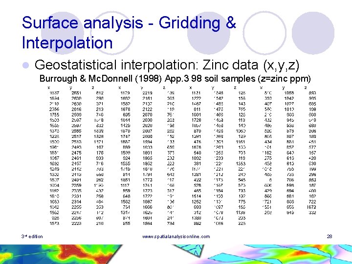
Surface analysis - Gridding & Interpolation l Geostatistical interpolation: Zinc data (x, y, z) Burrough & Mc. Donnell (1998) App. 3 98 soil samples (z=zinc ppm) 3 rd edition www. spatialanalysisonline. com 28

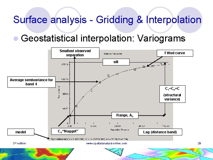
Surface analysis - Gridding & Interpolation l Geostatistical interpolation: Variograms Smallest observed separation Fitted curve sill Average semivariance for band 4 C 1=C 0+C (structural variance) Range, A 0 model 3 rd edition C 0 “Nugget” Lag (distance band) www. spatialanalysisonline. com 29

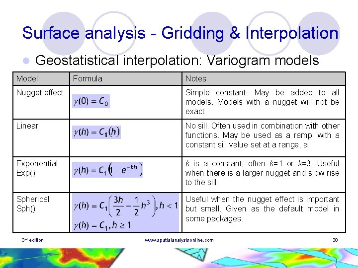
Surface analysis - Gridding & Interpolation l Geostatistical interpolation: Variogram models Model Formula Notes Nugget effect Simple constant. May be added to all models. Models with a nugget will not be exact Linear No sill. Often used in combination with other functions. May be used as a ramp, with a constant sill value set at a range, a Exponential Exp() k is a constant, often k=1 or k=3. Useful when there is a larger nugget and slow rise to the sill Spherical Sph() Useful when the nugget effect is important but small. Given as the default model in some packages. 3 rd edition www. spatialanalysisonline. com 30

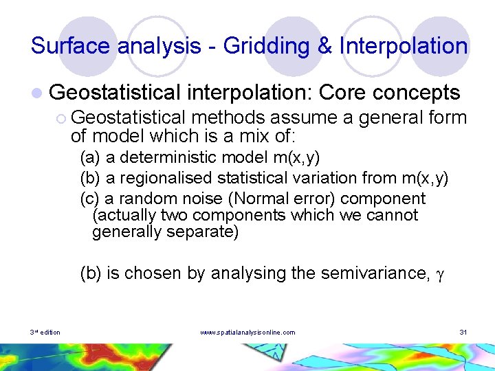
Surface analysis - Gridding & Interpolation l Geostatistical interpolation: Core concepts ¡ Geostatistical methods assume a general form of model which is a mix of: (a) a deterministic model m(x, y) (b) a regionalised statistical variation from m(x, y) (c) a random noise (Normal error) component (actually two components which we cannot generally separate) (b) is chosen by analysing the semivariance, 3 rd edition www. spatialanalysisonline. com 31

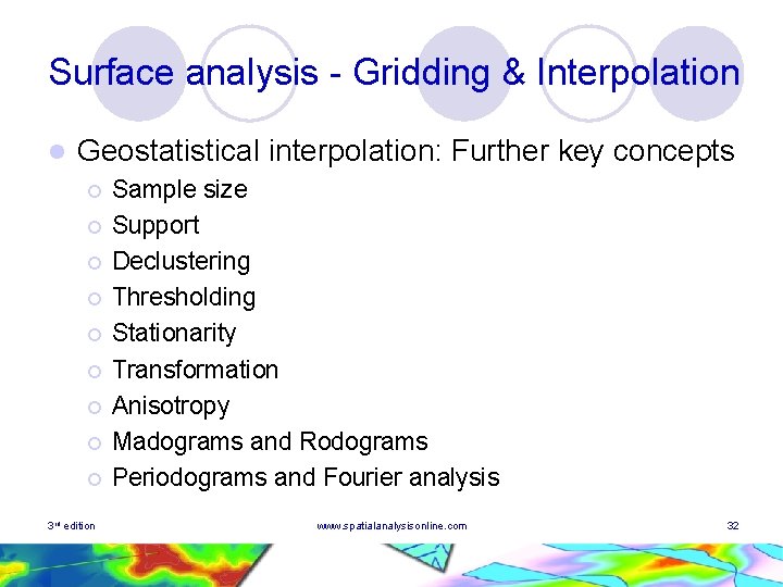
Surface analysis - Gridding & Interpolation l Geostatistical interpolation: Further key concepts ¡ ¡ ¡ ¡ ¡ 3 rd edition Sample size Support Declustering Thresholding Stationarity Transformation Anisotropy Madograms and Rodograms Periodograms and Fourier analysis www. spatialanalysisonline. com 32

Surface analysis - Gridding & Interpolation l Geostatistical interpolation: Kriging ¡ ¡ ¡ 3 rd edition Examine the data (z values) for spatial trends and Normality and transform variables if necessary, e. g. loge(z) or loge(z+1) Compute the experimental variogram and fit a suitable model IFF the pattern warrants this (i. e. the data is not just noise) Check the model by cross validation and examine size of mean squared deviation Decide on method to use – Kriging or Conditional simulation Generate a grid from the selected model and plot Compare the results to (a) the input data points and (b) other sources of data/information www. spatialanalysisonline. com 33

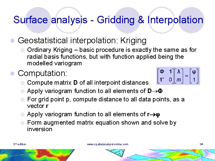
Surface analysis - Gridding & Interpolation l Geostatistical interpolation: Kriging ¡ l Ordinary Kriging – basic procedure is exactly the same as for radial basis functions, but with function applied being the modelled variogram Computation: ¡ ¡ ¡ 3 rd edition Compute matrix D of all interpoint distances Apply variogram function to all elements of D For grid point p, compute distance to all data points, as a vector r Apply variogram function to all elements of r Form augmented matrix equation shown and solve by inversion www. spatialanalysisonline. com 34

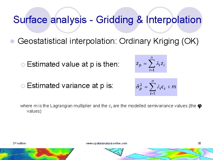
Surface analysis - Gridding & Interpolation l Geostatistical interpolation: Ordinary Kriging (OK) ¡ Estimated value at p is then: ¡ Estimated variance at p is: where m is the Lagrangian multiplier and the ci are the modelled semivariance values (the values) 3 rd edition www. spatialanalysisonline. com 35

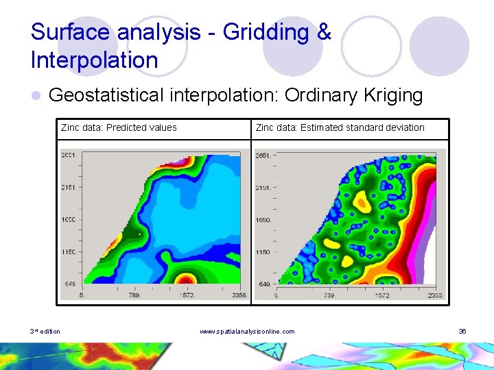
Surface analysis - Gridding & Interpolation l Geostatistical interpolation: Ordinary Kriging Zinc data: Predicted values 3 rd edition Zinc data: Estimated standard deviation www. spatialanalysisonline. com 36

Surface analysis - Gridding & Interpolation l Geostatistical ¡ Goodness interpolation: Kriging of fit methods: Residual plots, standard deviation plots l Examination for artefacts l Simple cross-validation l Jack-knifing l Re-sampling l Examination of independent datasets l Stratification l 3 rd edition www. spatialanalysisonline. com 37

Surface analysis - Gridding & Interpolation l Geostatistical interpolation: Kriging – other models ¡ Universal Kriging – Kriging with a trend ¡ Indicator Kriging – thresholding ¡ Stratified Kriging – regionalised approach ¡ Co-Kriging – use of associated data 3 rd edition www. spatialanalysisonline. com 38

Surface analysis - Gridding & Interpolation Geostatistical interpolation: Conditional simulation (Gaussian sequential method) l Similar to OK approach. 3 core steps: Analyse the data/transform as necessary, fit model variogram, define grid to use (possibly multi-level) 2. Randomly select a grid node to visit (e. g. apply a random walk process) as execute step 3 3. Apply OK estimation at node based on local observed data points. Take estimated value and apply Normal random process with mean as estimate and variance as estimated variance. Return to step 2 This process is then repeated until all nodes have been visited. Then iterated M times 1. 3 rd edition www. spatialanalysisonline. com 39

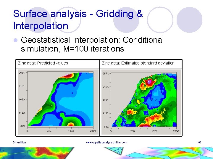
Surface analysis - Gridding & Interpolation l Geostatistical interpolation: Conditional simulation, M=100 iterations Zinc data: Predicted values 3 rd edition Zinc data: Estimated standard deviation www. spatialanalysisonline. com 40