Chapter 6 Open Methods Open Methods 6 1

Chapter 6 Open Methods

Open Methods • • • 6. 1 Simple Fixed-Point Iteration 6. 2 Newton-Raphson Method* 6. 3 Secant Methods* 6. 4 MATLAB function: fzero 6. 5 Polynomials

Open Methods • There exist open methods which do not require bracketed intervals • Newton-Raphson method, Secant Method, Muller’s method, fixed-point iterations • First one to consider is the fixed-point method • Converges faster but not necessary converges

Bracketing and Open Methods

Fixed-Point Iteration • First open method is fixed point iteration • Idea: rewrite original equation f(x) = 0 into another form x = g(x). • Use iteration xi+1 = g(xi ) to find a value that reaches convergence • Example:

Simple Fixed-Point Iteration f(x) = 0 Two Alternative Graphical Methods f 1(x) = f 2(x) f(x) = f 1(x) – f 2(x) = 0

Fixed. Point Iteration Convergent Divergent

Steps of Fixed-Point Iteration x = g(x), • Step f(x) = x - g(x) = 0 1: Guess x 0 and calculate y 0 = g(x 0). • Step 2: Let x 1 = g(x 0) • Step 3: Examining if x 1 is the solution of f(x) = 0. • Step 4. If not, repeat the iteration, x 0 = x 1

Newton’s Method • King of the root-finding methods • Newton-Raphson method • Based on Taylor series expansion

Newton-Raphson Method Truncate the Taylor series to get At the root, f(xi+1) = 0 , so

Newton-Raphson Method

Newton-Raphson Method False position - secant line Newton’s method - tangent line root x* xi+1 xi

Newton Raphson Method • Step 1: Start at the point (x 1, f(x 1)). • Step 2 : The intersection of the tangent of f(x) at this point and the x-axis. x 2 = x 1 - f(x 1)/f `(x 1) • Step 3: Examine if f(x 2) = 0 or abs(x 2 - x 1) < tolerance, • Step 4: If yes, solution xr = x 2 If not, x 1 x 2, repeat the iteration.

Newton’s Method • Note that an evaluation of the derivative (slope) is required • You may have to do this numerically • Open Method – Convergence depends on the initial guess (not guaranteed) • However, Newton method can converge very quickly (quadratic convergence)

Script file: Newtraph. m

Bungee Jumper Problem • Newton-Raphson method • Need to evaluate the function and its derivative Given cd = 0. 25 kg/m, v = 36 m/s, t = 4 s, and g = 9. 81 m 2/s, determine the mass of the bungee jumper

Bungee Jumper Problem >> y=inline('sqrt(9. 81*m/0. 25)*tanh(sqrt(9. 81*0. 25/m)*4)-36', 'm') y = Inline function: y(m) = sqrt(9. 81*m/0. 25)*tanh(sqrt(9. 81*0. 25/m)*4)-36 >> dy=inline('1/2*sqrt(9. 81/(m*0. 25))*tanh(sqrt(9. 81*0. 25/m)*4)9. 81/(2*m)*4*sech(sqrt(9. 81*0. 25/m)*4)^2', 'm') dy = Inline function: dy(m) = 1/2*sqrt(9. 81/(m*0. 25))*tanh(sqrt(9. 81*0. 25/m)*4)9. 81/(2*m)*4*sech(sqrt(9. 81*0. 25/m)*4)^2 >> format short; root = newtraph(y, dy, 140, 0. 00001) root = 142. 7376

Multiple Roots • A multiple root (double, triple, etc. ) occurs where the function is tangent to the x axis single root double roots

Examples of Multiple Roots

Multiple Roots • Problems with multiple roots • The function does not change sign at even multiple roots (i. e. , m = 2, 4, 6, …) • f (x) goes to zero - need to put a zero check for f(x) in program • slower convergence (linear instead of quadratic) of Newton-Raphson and secant methods for multiple roots

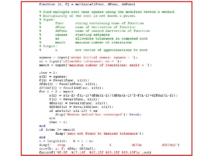
Modified Newton-Raphson Method • When the multiplicity of the root is known • Double root : m = 2 • Triple root : m = 3 • Simple, but need to know the multiplicity m • Maintain quadratic convergence See MATLAB solutions

Multiple Root with Multiplicity m f(x)=x 5 11 x 4 + 46 x 3 90 x 2 + 81 x 27 double root three roots Multiplicity m m = 1 : single root m = 2 : double root m = 3: triple root

Modified Newton’s Method Can be used for both single and multiple roots (m = 1: original Newton’s method) m =1: single root m=2, double root m=3 triple root etc.

Original Newton’s method m=1 » multiple 1('multi_func', 'multi_dfunc'); enter multiplicity of the root = 1 enter initial guess x 1 = 1. 3 allowable tolerance tol = 1. e-6 maximum number of iterations max = 100 Newton method has converged step x y 1 1. 30000000 -0. 44217000004 2 1. 096000000 -0. 063612622209021 3 1. 0440727272 -0. 014534428477418 4 1. 02126549372889 -0. 003503591972482 5 1. 01045853297516 -0. 000861391389428 6 1. 00518770530932 -0. 000213627276750 7 1. 00258369467652 -0. 000053197123947 8 1. 00128933592285 -0. 000013273393044 9 1. 00064404356011 -0. 000003315132176 10 1. 00032186610620 -0. 000000828382262 11 1. 00016089418619 -0. 000000207045531 12 1. 00008043738571 -0. 000000051755151 13 1. 00004021625682 -0. 000000012938003 14 1. 00002010751461 -0. 00003234405 15 1. 00001005358967 -0. 00000808605 16 1. 00000502663502 -0. 00000202135 17 1. 00000251330500 -0. 0000050527 18 1. 00000125681753 -0. 0000012626 19 1. 00000062892307 -0. 0000003162 Modified Newton’s Method m=2 » multiple 1('multi_func', 'multi_dfunc'); enter multiplicity of the root = 2 enter initial guess x 1 = 1. 3 allowable tolerance tol = 1. e-6 maximum number of iterations max = 100 Newton method has converged step x y 1 1. 30000000 -0. 44217000004 2 0. 891999999 -0. 109259530656779 3 0. 99229251101321 -0. 000480758689392 4 0. 99995587111371 -0. 000000015579900 5 0. 9999853944 -0. 00000007 6 1. 00000060664549 -0. 0000002935 Double root : m = 2 f(x) = x 5 11 x 4 + 46 x 3 90 x 2 + 81 x 27 = 0

Modified Newton’s Method with u = f / f • A more general modified Newton-Raphson method for multiple roots • u(x) contains only single roots even though f(x) may have multiple roots

Modified Newton’s method with u = f / f function f = multi_func(x) % Exact solutions: x = 1 (double) and 2 (triple) f = x. ^5 - 11*x. ^4 + 46*x. ^3 - 90*x. ^2 + 81*x - 27; function f_pr = multi_pr(x) % First derivative f'(x) f_pr = 5*x. ^4 - 44*x. ^3 + 138*x. ^2 - 180*x + 81; function f_pp = multi_pp(x) % Second-derivative f''(x) f_pp = 20*x. ^3 - 132*x. ^2 + 276*x - 180; >> [x, f] = multiple 2('multi_func', 'multi_ddfunc'); enter initial guess: xguess = 0 Double root allowable tolerance: es = 1. e-6 at x = 1 maximum number of iterations: maxit = 100 Newton method has converged step x f df/dx d 2 f/dx 2 1 0. 0000000 -27. 00000000 81. 00000000 -180. 00000000 2 1. 28571429 -0. 411257214255940 -2. 159100374843831 -0. 839650145772595 3 1. 080000002 -0. 045298483200014 -1. 061683200000175 -10. 690559999999067 4 1. 00519482 -0. 000214210129556 -0. 082148747927818 -15. 627914214305775 5 1. 00002034484531 -0. 00003311200 -0. 000325502624349 -15. 998535200938932 6 1. 0000031772 0. 00000000 -0. 00005083592 -15. 999999977123849 7 1. 0000031772 0. 00000000 -0. 00005083592 -15. 999999977123849

Original Newton’s method (m = 1) f(x) = x 5 11 x 4 + 46 x 3 90 x 2 + 81 x 27 = 0 >> [x, f] = multiple 1('multi_func', 'multi_dfunc'); enter multiplicity of the root = 1 enter initial guess: xguess = 10 Triple Root at x = 3 allowable tolerance: es = 1. e-6 maximum number of iterations: maxit = 200 Newton method has converged step x f df/dx 1 10. 0000000 27783. 00000000 18081. 00000000 2 8. 463414634 9083. 801268988610900 7422. 201416184873800 3 7. 23954576295397 2966. 633736828044700 3050. 171568370705200 4 6. 26693367529599 967. 245352637683710 1255. 503689063504700 5 5. 49652944545325 314. 604522684684700 517. 982397606370110 6 4. 88916416791005 101. 981559887686160 214. 391058318088990 7 4. 41348406871311 32. 905501521441806 89. 118850798301651 8 4. 04425240530314 10. 553044477409856 37. 250604948102705 9 3. 76095379868689 3. 358869623128157 15. 675199755246240 10 3. 54667457573766 1. 059579469957555 6. 646809147676663 … ……. . …… …. . 130 2. 99988506446967 -0. 0000006168 0. 000000158497869 131 2. 99992397673381 -0. 0000001762 0. 000000069347379 132 2. 99994938715307 -0. 000000426 0. 000000030737851 133 2. 99996325688118 -0. 000000085 0. 000000016199920 134 2. 99996852018682 0. 00000000 0. 000000011891075 135 2. 99996852018682 0. 00000000 0. 000000011891075

Modified Newton’s method f(x) = x 5 11 x 4 + 46 x 3 90 x 2 + 81 x 27 = 0 >> [x, f] = multiple 2('multi_func', 'multi_ddfunc'); enter initial guess: xguess = 10 allowable tolerance: es = 1. e-6 maximum number of iterations: maxit = 100 Triple root at x = 3 Newton method has converged step x f df/dx d 2 f/dx 2 1 10. 0000000 27783. 00000000 18081. 00000000 9380. 00000000 2 2. 42521994134897 -0. 385717068699165 1. 471933198691602 -1. 734685930313219 3 2. 80435435817775 -0. 024381150764611 0. 346832001230098 -3. 007964394244482 4 2. 98444590681717 -0. 000014818785758 0. 002843242444783 -0. 361760865258020 5 2. 99991809093254 -0. 0000002188 0. 000000080500286 -0. 001965495593481 6 2. 99999894615774 -0. 000000028 0. 0000013529 -0. 000025292161013 7 2. 99999841112323 0. 00000000 0. 0000030582 -0. 000038132921304 Ø Original Newton-Raphson method required 135 iterations Ø Modified Newton’s method converged in only 7 iterations

Convergence of Newton’s Method • The error of the Newton-Raphson method (for single root) can be estimated from xk+1 Quadratic convergence

Newton-Raphson Method Although Newton-Raphson converges very rapidly, it may diverge and fail to find roots 1) if an inflection point (f’’=0) is near the root 2) if there is a local minimum or maximum (f’=0) 3) if there are multiple roots 4) if a zero slope is reached Open Method, Convergence not guaranteed

Newton-Raphson Method Examples of poor convergence

Secant Method Ø Use secant line instead of tangent line at f(xi)

Secant Method • The formula for the secant method is • Notice that this is very similar to the false position method in form • Still requires two initial estimates • But it doesn't bracket the root at all times - there is no sign test

False-Position and Secant Methods

Algorithm for Secant method • Open Method 1. Begin with any two endpoints [a, b] = [x 0 , x 1] 2. Calculate x 2 using the secant method formula 3. Replace x 0 with x 1, replace x 1 with x 2 and repeat from (2) until convergence is reached • Use the two most recently generated points in subsequent iterations (not a bracket method!)

Secant Method • Advantage of the secant method • It can converge even faster and it doesn’t need to bracket the root • Disadvantage of the secant method • It is not guaranteed to converge! • It may diverge (fail to yield an answer)

Convergence not Guaranteed y = ln x no sign check, may not bracket the root

Secant method » [x 1 f 1]=secant('my_func', 0, 1, 1. e-15, 100); secant method has converged step x f 1. 0000 0 1. 0000 2. 0000 1. 0000 -1. 0000 3. 0000 0. 5000 -0. 3750 4. 0000 0. 2000 0. 4080 5. 0000 0. 3563 -0. 0237 6. 0000 0. 3477 -0. 0011 7. 0000 0. 3473 0. 0000 8. 0000 0. 3473 0. 0000 9. 0000 0. 3473 0. 0000 10. 0000 0. 3473 0. 0000 False position method » [x 2 f 2]=false_position('my_func', 0, 1, 1. e-15, 100); false_position method has converged step xl xu x f 1. 0000 0. 5000 -0. 3750 2. 0000 0 0. 5000 0. 3636 -0. 0428 3. 0000 0 0. 3636 0. 3487 -0. 0037 4. 0000 0 0. 3487 0. 3474 -0. 0003 5. 0000 0 0. 3474 0. 3473 0. 0000 6. 0000 0 0. 3473 0. 0000 7. 0000 0 0. 3473 0. 0000 8. 0000 0 0. 3473 0. 0000 9. 0000 0 0. 3473 0. 0000 10. 0000 0 0. 3473 0. 0000 11. 0000 0 0. 3473 0. 0000 12. 0000 0 0. 3473 0. 0000 13. 0000 0 0. 3473 0. 0000 14. 0000 0 0. 3473 0. 0000 15. 0000 0 0. 3473 0. 0000 16. 0000 0 0. 3473 0. 0000

Secant method may converge even faster and it doesn’t need to bracket the root Secant method False position

Similarity & Difference b/w F-P & Secant Methods False-point method Secant method • Starting two points. • Similar formula xm = xu - f(xu)(xu-xl)/(f(xu)- f(xl)) ______________ • Next iteration: points replacement: if f(xm)*f(xl) <0, then xu = xm else xl = xm. • Require bracketing. x 3= x 2 -f(x 2)(x 2 -x 1)/(f(x 2)- f(x 1)) ______________ • Next iteration: points replacement: always x 1 = x 2 & x 2 =x 3. • no requirement of bracketing. • Faster convergence • May not converge • Always converge

Convergence criterion 10 -14 Bisection -47 iterations False position -- 15 iterations Secant -10 iterations Newton’s -6 iterations False position Secant Newton’s Bisection

Modified Secant Method • Use fractional perturbation instead of two arbitrary values to estimate the derivative • is a small perturbation fraction (e. g. , xi/xi = 10 6)

MATLAB Function: fzero • Bracketing methods – reliable but slow • Open methods – fast but possibly unreliable • MATLAB fzero – fast and reliable • fzero: find real root of an equation (not suitable for double root!) fzero(function, x 0) fzero(function, [x 0 x 1])

>> root=fzero('multi_func', -10) fzero unable to find the double root of root = f(x) = x 5 11 x 4 + 46 x 3 90 x 2 + 81 x 27 = 0 2. 99997215011186 >> root=fzero('multi_func', 1000) root = 2. 99996892915965 >> root=fzero('multi_func', [-1000]) root = 2. 99998852581534 >> root=fzero('multi_func', [-2 2]) ? ? ? Error using ==> fzero The function values at the interval endpoints must differ in sign. >> root=multiple 2('multi_func', 'multi_ddfunc'); enter initial guess: xguess = -1 allowable tolerance: es = 1. e-6 maximum number of iterations: maxit = 100 Newton method has converged step x 1 -1. 0000000 2 1. 54545455 3 1. 34838709677419 4 1. 12513231297383 5 1. 01327476262380 6 1. 00013392759869 7 1. 00000001342083 8 1. 00000001342083 f -256. 00000000 -0. 915585746130091 -0. 546825709009667 -0. 103193137485462 -0. 001381869252874 -0. 000000143464007 0. 000000000000000 df/dx d 2 f/dx 2 448. 00000000 -608. 00000000 -1. 468752134417059 5. 096919609316331 -2. 145926990290406 1. 190673693397343 -1. 484223690473826 -8. 078669685137726 -0. 206108293568889 -15. 056858096928863 -0. 002142195919063 -15. 990358504281403 -0. 000000214733291 -15. 999999033700192

fzero and optimset functions >> options=optimset('display', 'iter'); >> [x fx]=fzero('manning', 50, options) Func-count x f(x) 1 50 -14569. 8 2 48. 5858 -14062 3 51. 4142 -15078. 3 4 48 -13851. 9 5 52 -15289. 1. . . 18 19 20 21 22 . . . 27. 3726 72. 6274 18 82 4. 74517 Procedure initial search Search in both search directions x 0 x search for sign change . . . -6587. 13 -22769. 2 -3457. 1 -26192. 5 319. 67 search search Find sign change after 22 iterations Looking for a zero in the interval [4. 7452, 82] 23 5. 67666 110. 575 interpolation 24 6. 16719 -5. 33648 interpolation 25 6. 14461 0. 0804104 interpolation 26 6. 14494 5. 51498 e-005 interpolation 27 6. 14494 -1. 47793 e-012 interpolation 28 6. 14494 3. 41061 e-013 interpolation 29 6. 14494 -5. 68434 e-013 interpolation Zero found in the interval: [4. 7452, 82]. x = 6. 14494463443476 Switch to secant (linear) or inverse fx = quadratic interpolation to find root 3. 410605131648481 e-013

Root of Polynomials • Bisection, false-position, Newton-Raphson, secant methods cannot be easily used to determine all roots of higher-order polynomials • Muller’s method (Chapra and Canale, 2002) • Bairstow method (Chapra and Canale, 2002) • MATLAB function: roots

Secant and Muller’s Method

Muller’s Method y(x) Secant line x 1 x 3 x 2 x Parabola Ø Fit a parabola (quadratic) to exact curve Ø Find both real and complex roots (x 2 + rx + s = 0 )

MATLAB Function: roots • Recast the root evaluation task as an eigenvalue problem (Chapter 20) • Zeros of a nth-order polynomial r = roots(c) - roots c = poly(r) - inverse function

Roots of Polynomial • Consider the 6 th-order polynomial (4 real and 2 complex roots) >> c = [1 -6 14 10 -111 56 156]; >> r = roots(c) r = 2. 0000 + 3. 0000 i 2. 0000 - 3. 0000 i 3. 0000 2. 0000 -1. 0000 >> polyval(c, r), format long g ans = 1. 36424205265939 e-012 + 4. 50484094471904 e-012 i 1. 36424205265939 e-012 - 4. 50484094471904 e-012 i -1. 30739863379858 e-012 1. 4210854715202 e-013 7. 105427357601 e-013 Verify f(xr) =0 5. 6843418860808 e-014

f(x) = x 5 11 x 4 + 46 x 3 90 x 2 + 81 x 27 = (x 1)2(x 3)3 >> c = [1 -11 46 -90 81 -27]; r = roots(c) r = 3. 00003350708868 2. 99998324645566 + 0. 00002901794688 i 2. 99998324645566 - 0. 00002901794688 i 1. 0000000 + 0. 00000003325168 i 1. 0000000 - 0. 00000003325168 i

CVEN 302 -501 Homework No. 5 • Chapter 5 • Problem 5. 10 b) & c) (25)(using MATLAB Programs) • Chapter 6 • Problem 6. 3 (Hand Calculations for parts (b), (c), (d))(25) • Problem 6. 7 (MATLAB Program) (25) • Problem 6. 9 (MATLAB program) (25) • Problem 6. 16 (use MATLAB function fzero) (25) • Due on Monday 09/29/08 at the beginning of the period