Chapter 6 Numerical Interpolation Given some sample measurements

Chapter 6 Numerical Interpolation • Given some sample measurements, we may need to estimate the values at some other points by fitting a curve to the measured points. • Interpolation is required in many engineering applications that use tabular data as input. • The basis of all interpolation algorithms is the fitting of some type of curve or function to a subset of the tabular data. 1

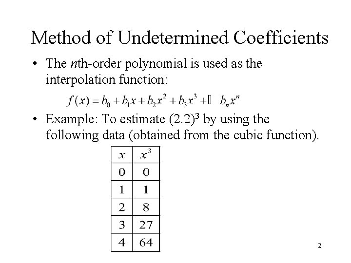
Method of Undetermined Coefficients • The nth-order polynomial is used as the interpolation function: • Example: To estimate (2. 2)3 by using the following data (obtained from the cubic function). 2

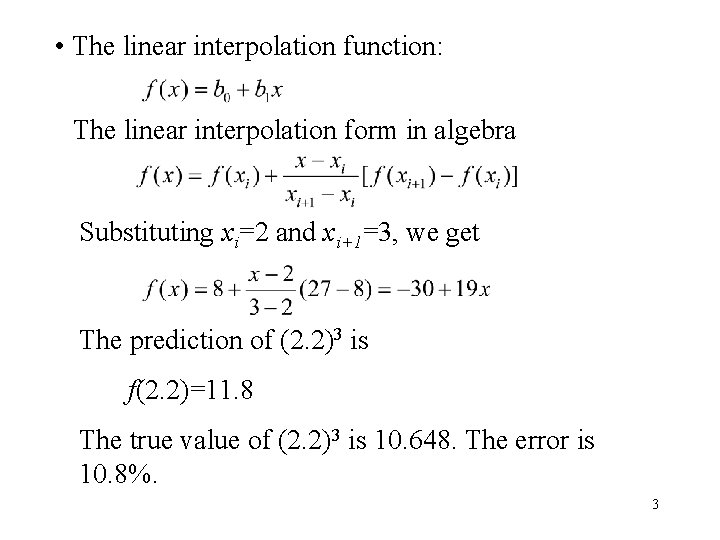
• The linear interpolation function: The linear interpolation form in algebra Substituting xi=2 and xi+1=3, we get The prediction of (2. 2)3 is f(2. 2)=11. 8 The true value of (2. 2)3 is 10. 648. The error is 10. 8%. 3

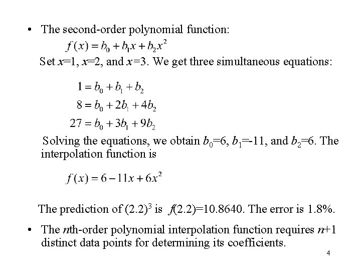
• The second-order polynomial function: Set x=1, x=2, and x=3. We get three simultaneous equations: Solving the equations, we obtain b 0=6, b 1=-11, and b 2=6. The interpolation function is The prediction of (2. 2)3 is f(2. 2)=10. 8640. The error is 1. 8%. • The nth-order polynomial interpolation function requires n+1 distinct data points for determining its coefficients. 4

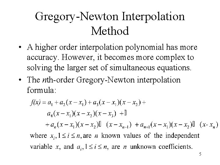
Gregory-Newton Interpolation Method • A higher order interpolation polynomial has more accuracy. However, it becomes more complex to solving the larger set of simultaneous equations. • The nth-order Gregory-Newton interpolation formula: 5

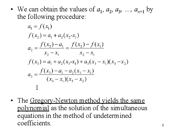
• We can obtain the values of a 1, a 2, a 3, …, an+1 by the following procedure: • The Gregory-Newton method yields the same polynomial as the solution of the simultaneous equations in the method of undetermined coefficients. 6

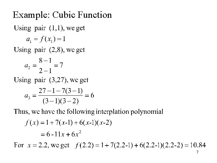
Example: Cubic Function 7

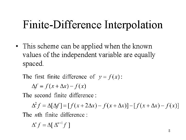
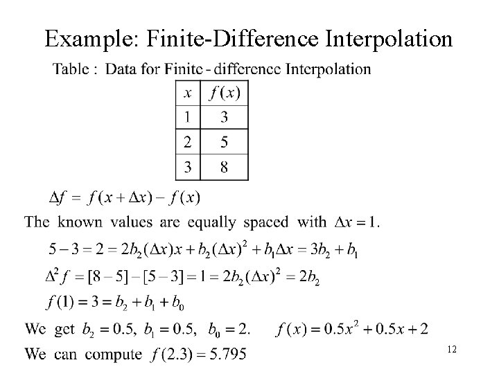
Finite-Difference Interpolation • This scheme can be applied when the known values of the independent variable are equally spaced. 8

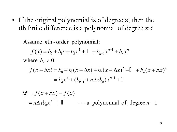
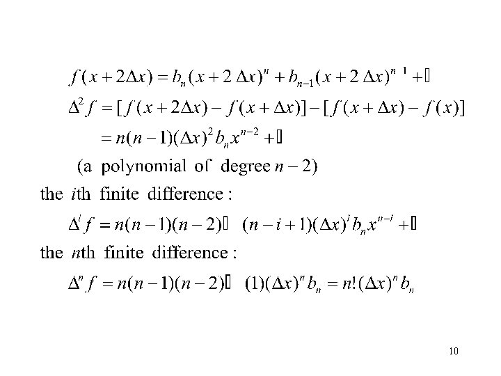
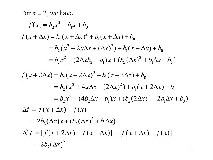
• If the original polynomial is of degree n, then the ith finite difference is a polynomial of degree n-i. 9

10

11

Example: Finite-Difference Interpolation 12

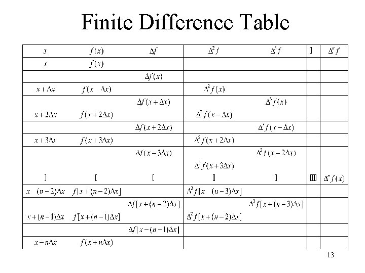
Finite Difference Table 13

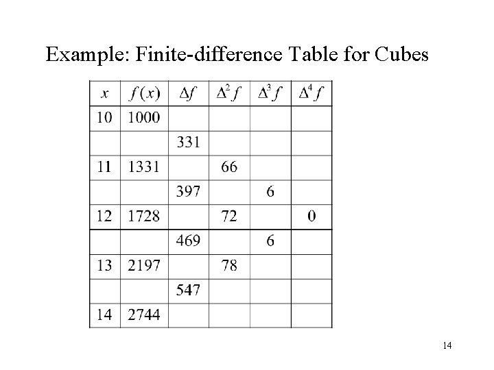
Example: Finite-difference Table for Cubes 14

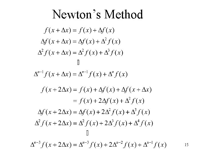
Newton’s Method 15

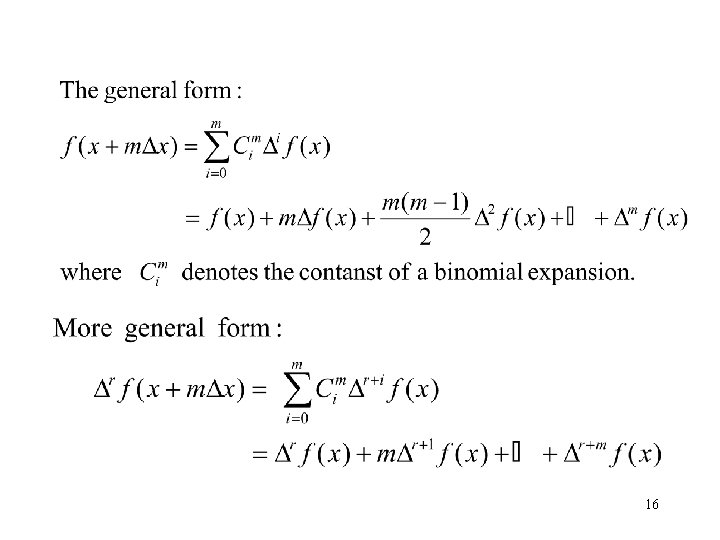
16

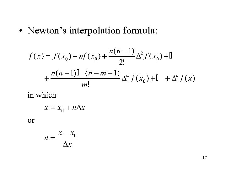
• Newton’s interpolation formula: 17

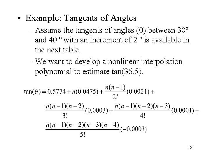
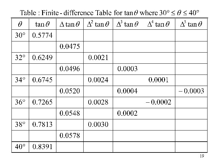
• Example: Tangents of Angles – Assume the tangents of angles ( ) between 30º and 40 º with an increment of 2 º is available in the next table. – We want to develop a nonlinear interpolation polynomial to estimate tan(36. 5). 18

19

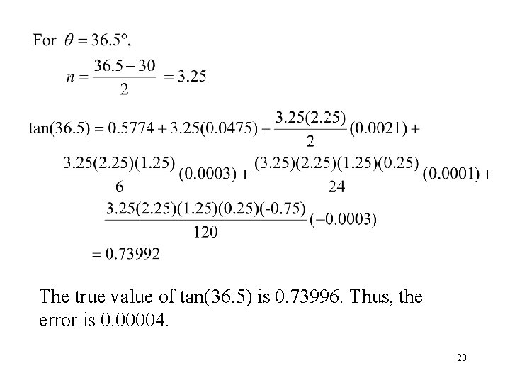
The true value of tan(36. 5) is 0. 73996. Thus, the error is 0. 00004. 20

Lagrange Polynomials • In Newton’s method, it is assumed that x is measured at a constant interval, x. • In Lagrange’s method, x is measured on a variable interval x. 21

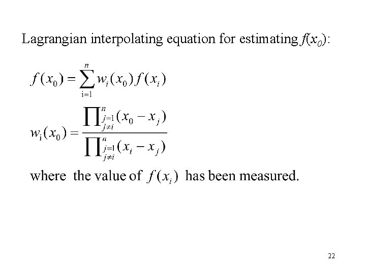
Lagrangian interpolating equation for estimating f(x 0): 22

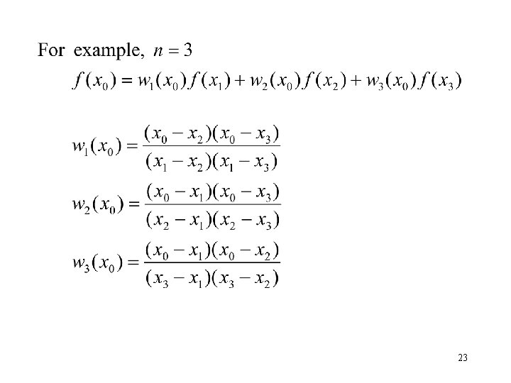
23

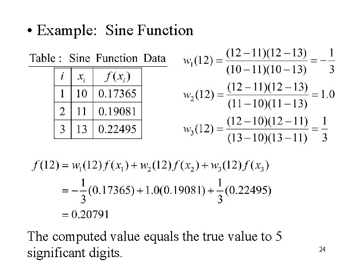
• Example: Sine Function The computed value equals the true value to 5 significant digits. 24

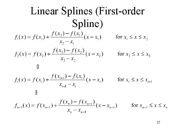
Linear Splines (First-order Spline) 25

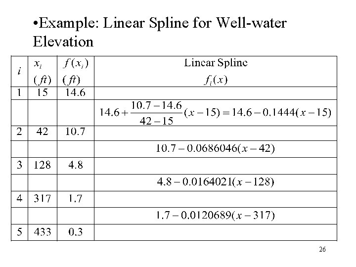
• Example: Linear Spline for Well-water Elevation 26

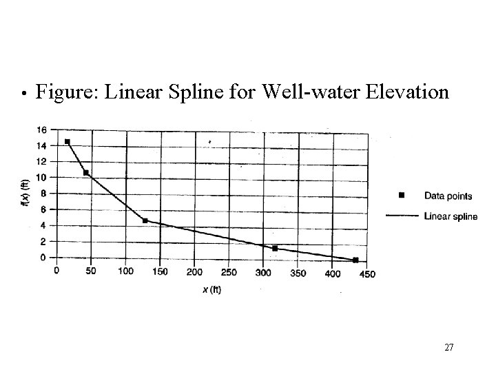
• Figure: Linear Spline for Well-water Elevation 27

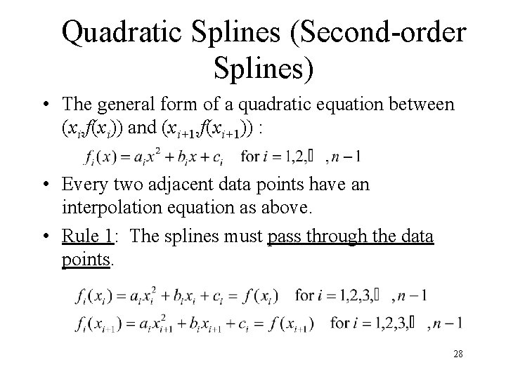
Quadratic Splines (Second-order Splines) • The general form of a quadratic equation between (xi, f(xi)) and (xi+1, f(xi+1)) : • Every two adjacent data points have an interpolation equation as above. • Rule 1: The splines must pass through the data points. 28

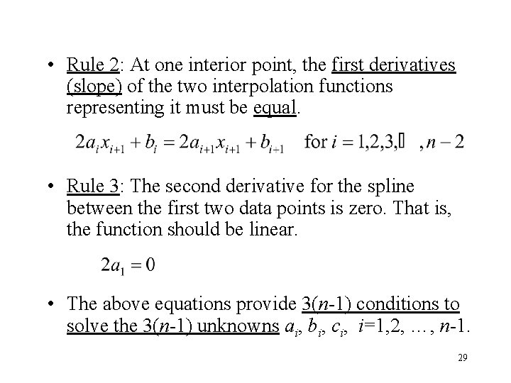
• Rule 2: At one interior point, the first derivatives (slope) of the two interpolation functions representing it must be equal. • Rule 3: The second derivative for the spline between the first two data points is zero. That is, the function should be linear. • The above equations provide 3(n-1) conditions to solve the 3(n-1) unknowns ai, bi, ci, i=1, 2, …, n-1. 29

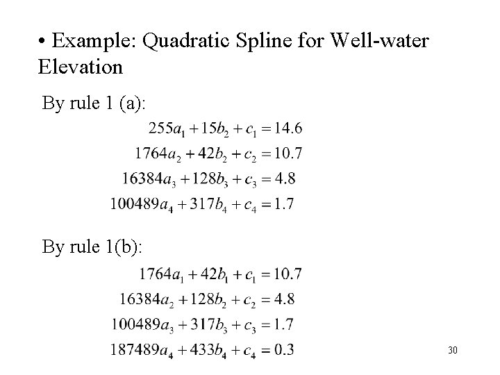
• Example: Quadratic Spline for Well-water Elevation By rule 1 (a): By rule 1(b): 30

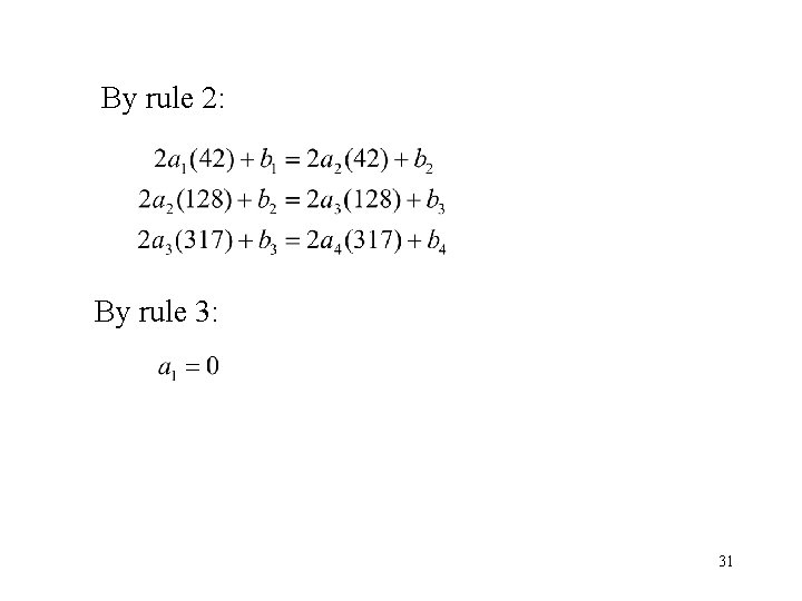
By rule 2: By rule 3: 31

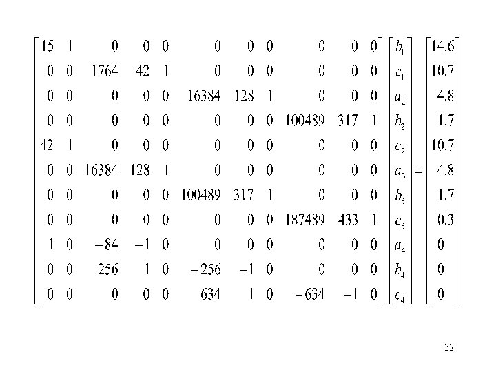
32

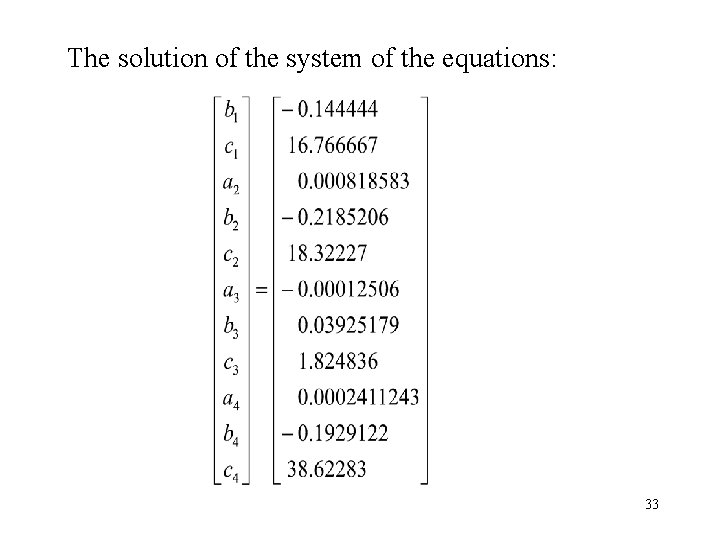
The solution of the system of the equations: 33

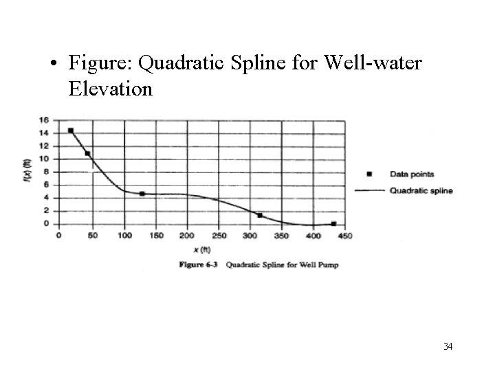
• Figure: Quadratic Spline for Well-water Elevation 34

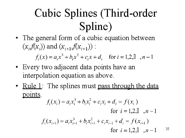
Cubic Splines (Third-order Spline) • The general form of a cubic equation between (xi, f(xi)) and (xi+1, f(xi+1)) : • Every two adjacent data points have an interpolation equation as above. • Rule 1: The splines must pass through the data points. 35

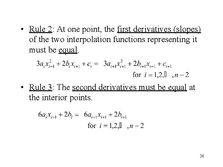
• Rule 2: At one point, the first derivatives (slopes) of the two interpolation functions representing it must be equal. • Rule 3: The second derivatives must be equal at the interior points. 36

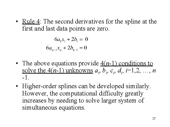
• Rule 4: The second derivatives for the spline at the first and last data points are zero. • The above equations provide 4(n-1) conditions to solve the 4(n-1) unknowns ai, bi, ci, di, i=1, 2, …, n -1. • Higher-order splines can be developed similarly. However, the computational difficulty greatly increases by needing to solve larger system of simultaneous equations. 37

Guidelines for Choice of Interpolation Method • The method of undetermined coefficients is perhaps the easiest method to understand conceptually. However, the method does require the solution of a set of n+1 simultaneous equations for an nth-order interpolation polynomial. One advantage of this method is that the interpolation polynomial can be customized for the particular problem at hand; for example, some of the terms of the general nth-order interpolation polynomial can be dropped, if desired. This is not possible in most of the other interpolation methods. 38

• Both the Gregory-Newton and Lagrange polynomial interpolation methods eliminate the need to solve a set of simultaneous equations. Of the two methods, the Lagrange polynomial scheme is perhaps the easier to program. Although both of these methods (as well as the method of undetermined coefficients) work with unequally spaced data points, the best accuracy is usually achieved when the differences in the spacing of the data points are minimal. • The finite-difference interpolation scheme requires equally spaced data points for its application. • Interpolation using splines can be more accurate than other methods, especially in cases where the data show large sudden changes. • All the interpolation schemes can also be used for extrapolation; but the accuracy usually becomes worse. 39

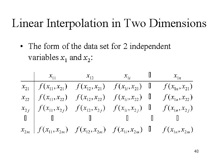
Linear Interpolation in Two Dimensions • The form of the data set for 2 independent variables x 1 and x 2: 40

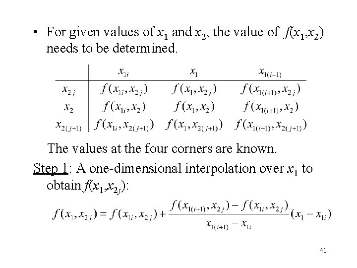
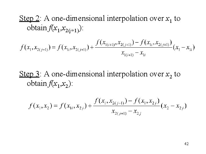
• For given values of x 1 and x 2, the value of f(x 1, x 2) needs to be determined. The values at the four corners are known. Step 1: A one-dimensional interpolation over x 1 to obtain f(x 1, x 2 j): 41

Step 2: A one-dimensional interpolation over x 1 to obtain f(x 1, x 2(j+1)): Step 3: A one-dimensional interpolation over x 2 to obtain f(x 1, x 2): 42