Chapter 6 Multiple Linear Regression Data Mining for

Chapter 6: Multiple Linear Regression Data Mining for Business Analytics in R (c) 2017 Shmueli, Bruce, Yahav & Patel © Galit Shmueli and Peter Bruce 2017

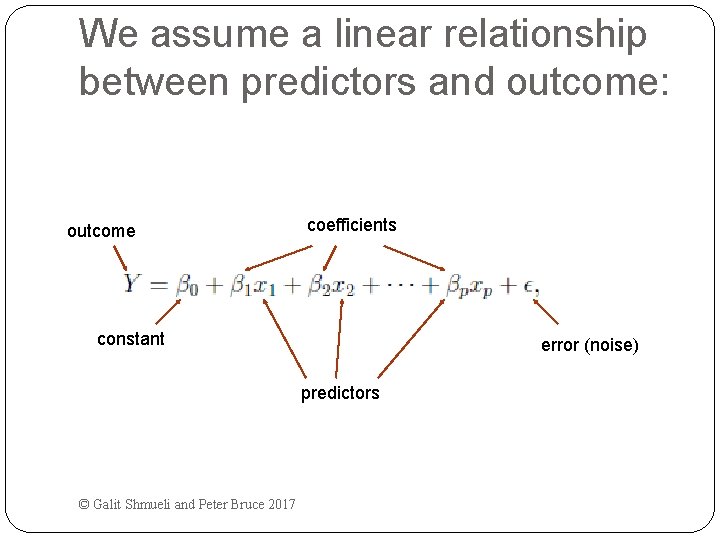
We assume a linear relationship between predictors and outcome: outcome coefficients constant error (noise) predictors © Galit Shmueli and Peter Bruce 2017

Topics Explanatory vs. predictive modeling with regression Example: prices of Toyota Corollas Fitting a predictive model Assessing predictive accuracy Selecting a subset of predictors © Galit Shmueli and Peter Bruce 2017

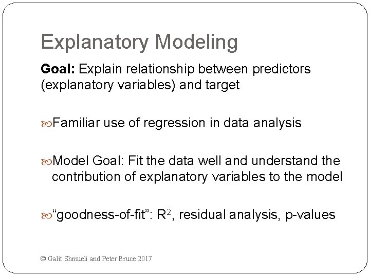
Explanatory Modeling Goal: Explain relationship between predictors (explanatory variables) and target Familiar use of regression in data analysis Model Goal: Fit the data well and understand the contribution of explanatory variables to the model “goodness-of-fit”: R 2, residual analysis, p-values © Galit Shmueli and Peter Bruce 2017

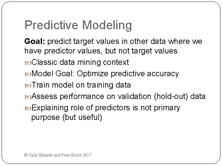
Predictive Modeling Goal: predict target values in other data where we have predictor values, but not target values Classic data mining context Model Goal: Optimize predictive accuracy Train model on training data Assess performance on validation (hold-out) data Explaining role of predictors is not primary purpose (but useful) © Galit Shmueli and Peter Bruce 2017

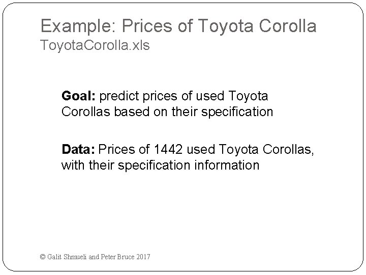
Example: Prices of Toyota Corolla Toyota. Corolla. xls Goal: predict prices of used Toyota Corollas based on their specification Data: Prices of 1442 used Toyota Corollas, with their specification information © Galit Shmueli and Peter Bruce 2017

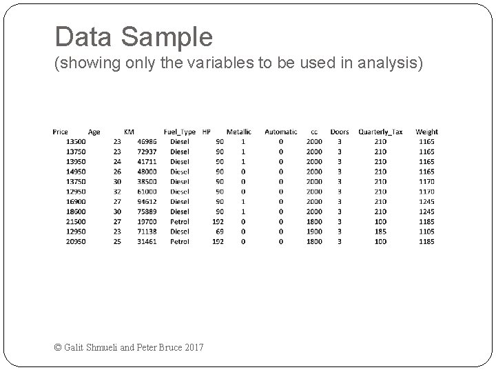
Data Sample (showing only the variables to be used in analysis) © Galit Shmueli and Peter Bruce 2017

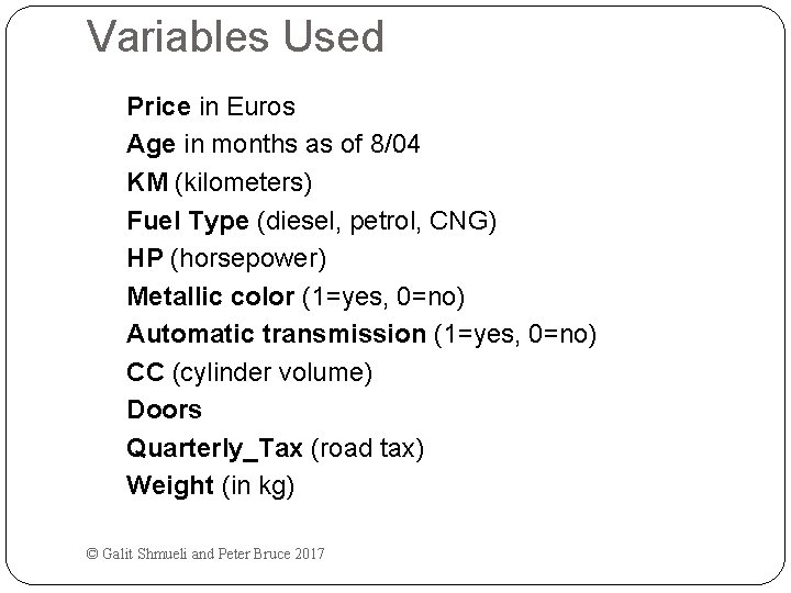
Variables Used Price in Euros Age in months as of 8/04 KM (kilometers) Fuel Type (diesel, petrol, CNG) HP (horsepower) Metallic color (1=yes, 0=no) Automatic transmission (1=yes, 0=no) CC (cylinder volume) Doors Quarterly_Tax (road tax) Weight (in kg) © Galit Shmueli and Peter Bruce 2017

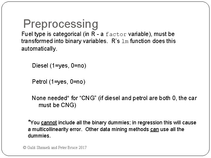
Preprocessing Fuel type is categorical (in R - a factor variable), must be transformed into binary variables. R’s lm function does this automatically. Diesel (1=yes, 0=no) Petrol (1=yes, 0=no) None needed* for “CNG” (if diesel and petrol are both 0, the car must be CNG) *You cannot include all the binary dummies; in regression this will cause a multicollinearity error. Other data mining methods can use all the dummies. © Galit Shmueli and Peter Bruce 2017

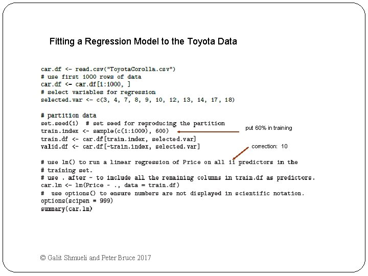
Fitting a Regression Model to the Toyota Data put 60% in training correction: 10 © Galit Shmueli and Peter Bruce 2017

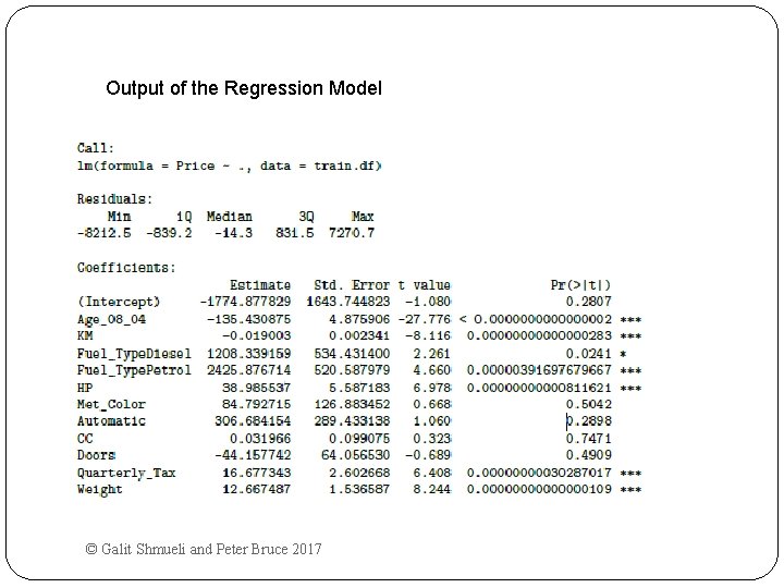
Output of the Regression Model © Galit Shmueli and Peter Bruce 2017

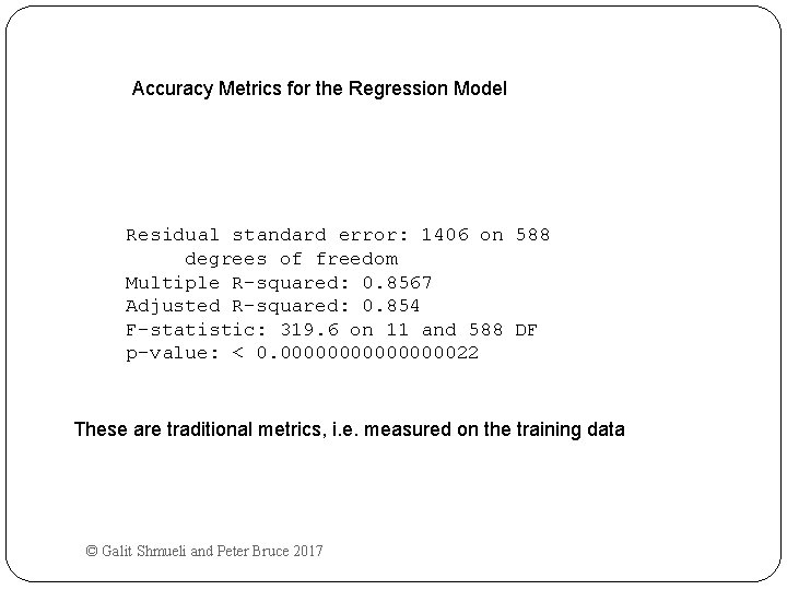
Accuracy Metrics for the Regression Model Residual standard error: 1406 on 588 degrees of freedom Multiple R-squared: 0. 8567 Adjusted R-squared: 0. 854 F-statistic: 319. 6 on 11 and 588 DF p-value: < 0. 0000000022 These are traditional metrics, i. e. measured on the training data © Galit Shmueli and Peter Bruce 2017

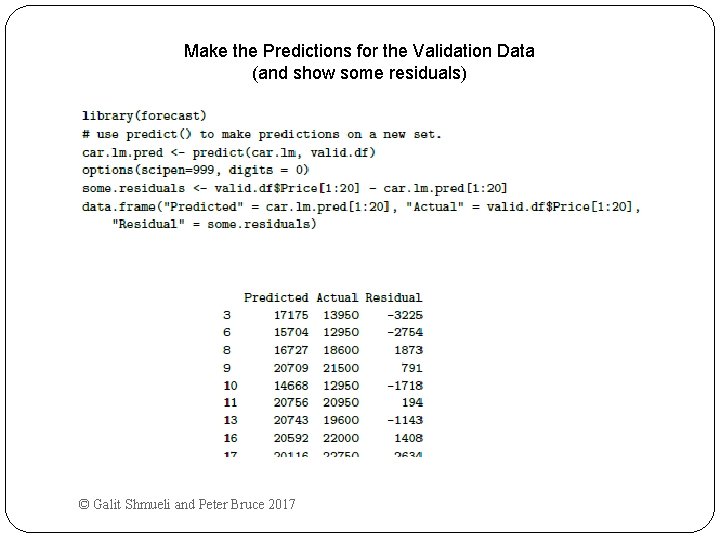
Make the Predictions for the Validation Data (and show some residuals) © Galit Shmueli and Peter Bruce 2017

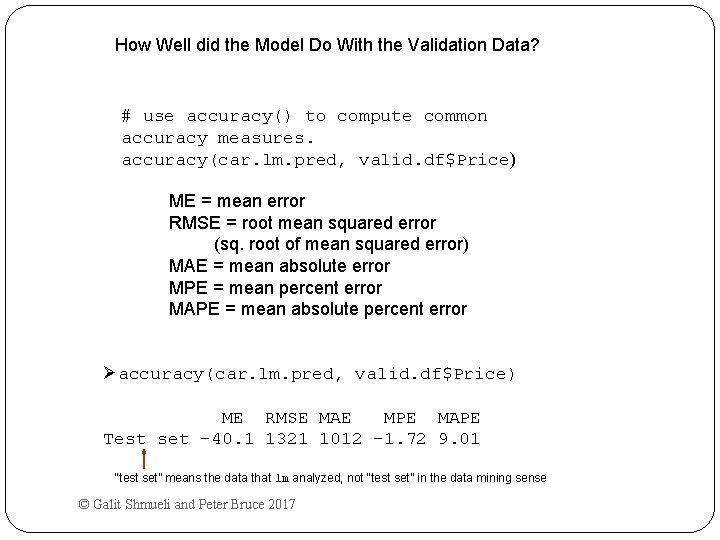
How Well did the Model Do With the Validation Data? # use accuracy() to compute common accuracy measures. accuracy(car. lm. pred, valid. df$Price) ME = mean error RMSE = root mean squared error (sq. root of mean squared error) MAE = mean absolute error MPE = mean percent error MAPE = mean absolute percent error Øaccuracy(car. lm. pred, valid. df$Price) ME RMSE MAE MPE MAPE Test set -40. 1 1321 1012 -1. 72 9. 01 “test set” means the data that lm analyzed, not “test set” in the data mining sense © Galit Shmueli and Peter Bruce 2017

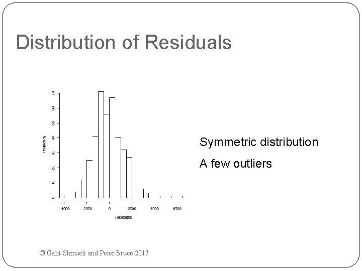
Distribution of Residuals Symmetric distribution A few outliers © Galit Shmueli and Peter Bruce 2017

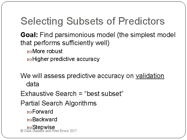
Selecting Subsets of Predictors Goal: Find parsimonious model (the simplest model that performs sufficiently well) More robust Higher predictive accuracy We will assess predictive accuracy on validation data Exhaustive Search = “best subset” Partial Search Algorithms Forward Backward Stepwise © Galit Shmueli and Peter Bruce 2017

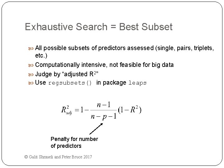
Exhaustive Search = Best Subset All possible subsets of predictors assessed (single, pairs, triplets, etc. ) Computationally intensive, not feasible for big data Judge by “adjusted R 2” Use regsubsets() in package leaps Penalty for number of predictors © Galit Shmueli and Peter Bruce 2017

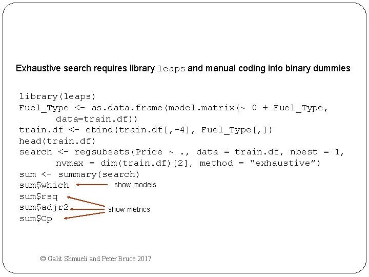
Exhaustive search requires library leaps and manual coding into binary dummies library(leaps) Fuel_Type <- as. data. frame(model. matrix(~ 0 + Fuel_Type, data=train. df)) train. df <- cbind(train. df[, -4], Fuel_Type[, ]) head(train. df) search <- regsubsets(Price ~. , data = train. df, nbest = 1, nvmax = dim(train. df)[2], method = “exhaustive”) sum <- summary(search) show models sum$which sum$rsq sum$adjr 2 show metrics sum$Cp © Galit Shmueli and Peter Bruce 2017

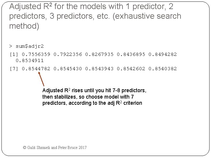
Adjusted R 2 for the models with 1 predictor, 2 predictors, 3 predictors, etc. (exhaustive search method) > sum$adjr 2 [1] 0. 7556359 0. 7922356 0. 8267935 0. 8436895 0. 8494282 0. 8534911 [7] 0. 8544782 0. 8545430 0. 8543943 0. 8542602 0. 8540382 Adjusted R 2 rises until you hit 7 -8 predictors, then stabilizes, so choose model with 7 predictors, according to the adj R 2 criterion © Galit Shmueli and Peter Bruce 2017

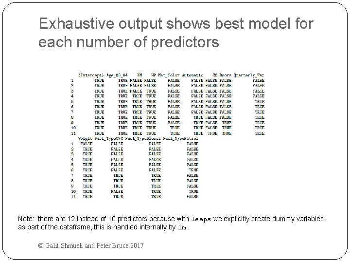
Exhaustive output shows best model for each number of predictors Note: there are 12 instead of 10 predictors because with leaps we explicitly create dummy variables as part of the dataframe, this is handled internally by lm. © Galit Shmueli and Peter Bruce 2017

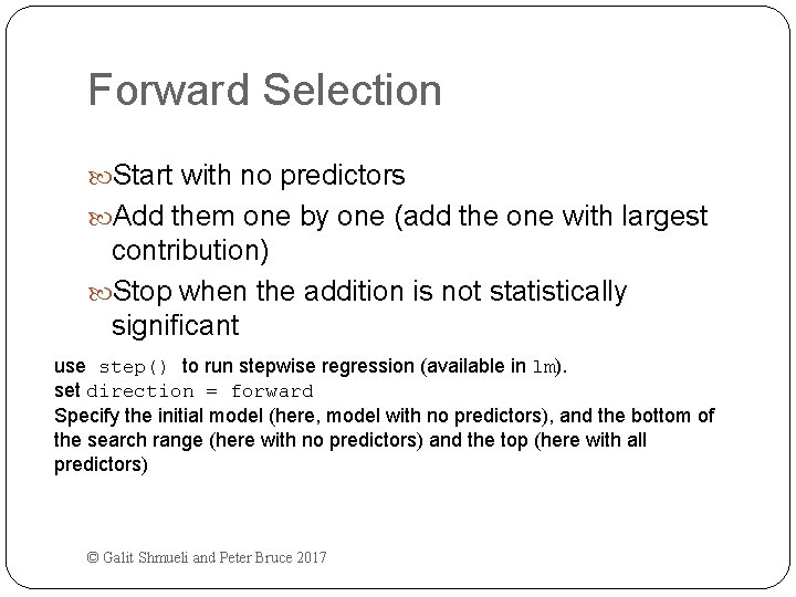
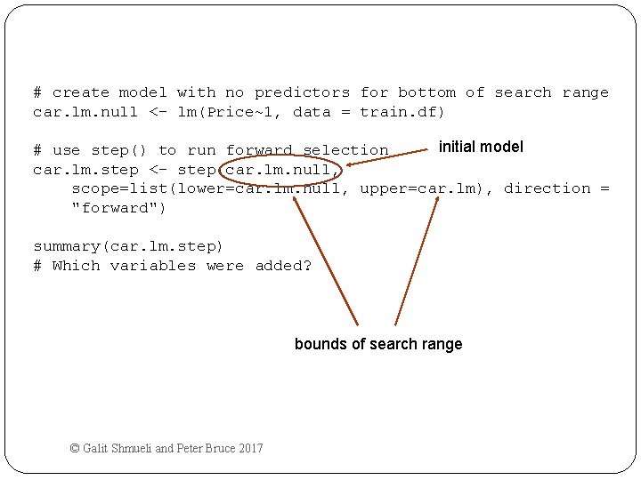
Forward Selection Start with no predictors Add them one by one (add the one with largest contribution) Stop when the addition is not statistically significant use step() to run stepwise regression (available in lm). set direction = forward Specify the initial model (here, model with no predictors), and the bottom of the search range (here with no predictors) and the top (here with all predictors) © Galit Shmueli and Peter Bruce 2017

# create model with no predictors for bottom of search range car. lm. null <- lm(Price~1, data = train. df) initial model # use step() to run forward selection car. lm. step <- step(car. lm. null, scope=list(lower=car. lm. null, upper=car. lm), direction = "forward") summary(car. lm. step) # Which variables were added? bounds of search range © Galit Shmueli and Peter Bruce 2017

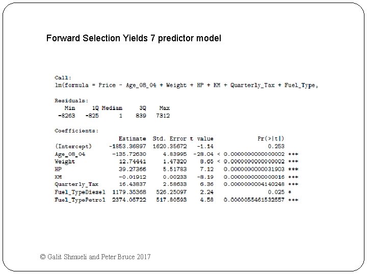
Forward Selection Yields 7 predictor model © Galit Shmueli and Peter Bruce 2017

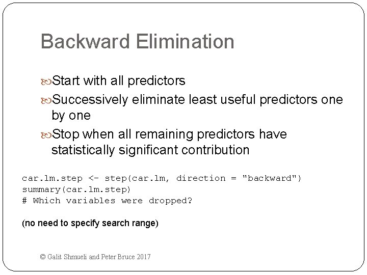
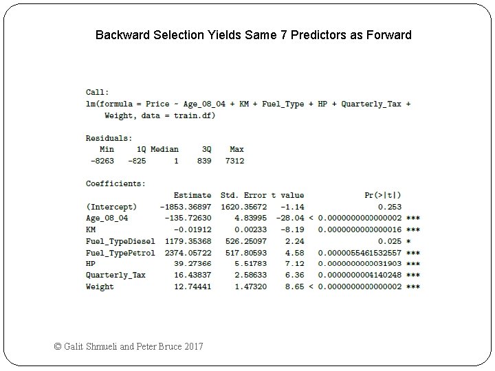
Backward Elimination Start with all predictors Successively eliminate least useful predictors one by one Stop when all remaining predictors have statistically significant contribution car. lm. step <- step(car. lm, direction = "backward") summary(car. lm. step) # Which variables were dropped? (no need to specify search range) © Galit Shmueli and Peter Bruce 2017

Backward Selection Yields Same 7 Predictors as Forward © Galit Shmueli and Peter Bruce 2017

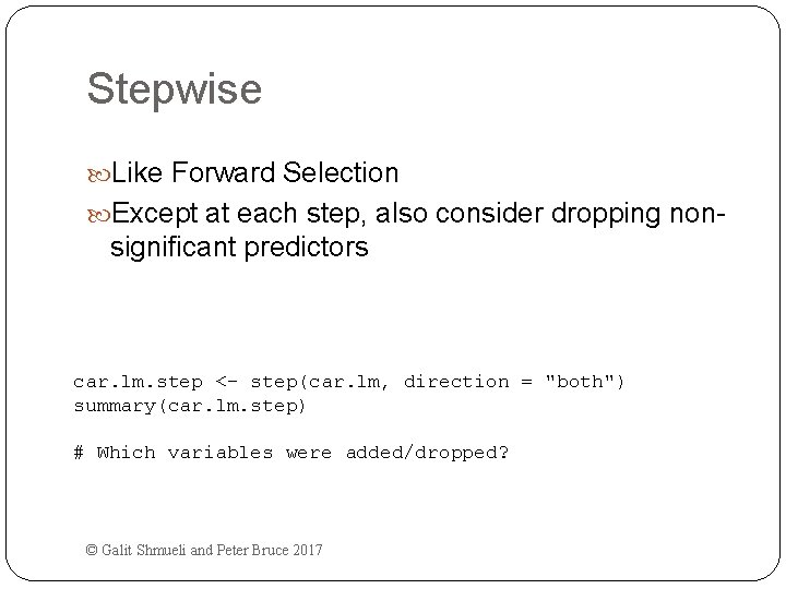
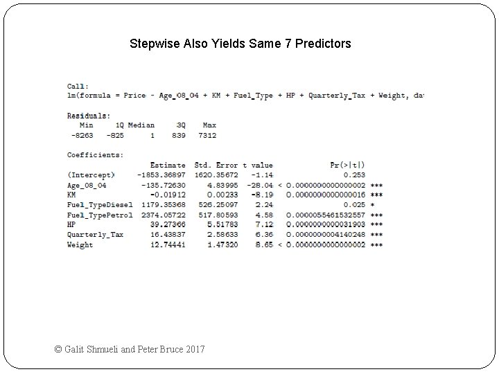
Stepwise Like Forward Selection Except at each step, also consider dropping non- significant predictors car. lm. step <- step(car. lm, direction = "both") summary(car. lm. step) # Which variables were added/dropped? © Galit Shmueli and Peter Bruce 2017

Stepwise Also Yields Same 7 Predictors © Galit Shmueli and Peter Bruce 2017

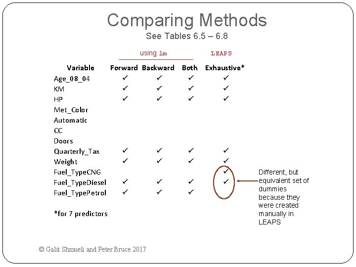
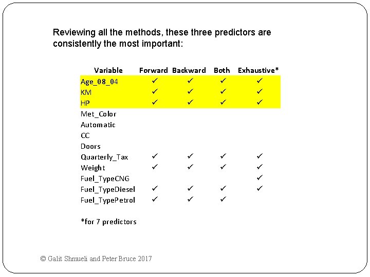
Comparing Methods See Tables 6. 5 – 6. 8 using lm LEAPS Variable Forward Backward Both Exhaustive* Age_08_04 ü ü KM ü ü HP ü ü Met_Color Automatic CC Doors Quarterly_Tax ü ü Weight ü ü Fuel_Type. CNG ü Fuel_Type. Diesel ü ü Fuel_Type. Petrol ü ü ü *for 7 predictors © Galit Shmueli and Peter Bruce 2017 Different, but equivalent set of dummies because they were created manually in LEAPS

Reviewing all the methods, these three predictors are consistently the most important: Variable Forward Backward Both Exhaustive* Age_08_04 ü ü KM ü ü HP ü ü Met_Color Automatic CC Doors Quarterly_Tax ü ü Weight ü ü Fuel_Type. CNG ü Fuel_Type. Diesel ü ü Fuel_Type. Petrol ü ü ü *for 7 predictors © Galit Shmueli and Peter Bruce 2017

Summary Linear regression models are very popular tools, not only for explanatory modeling, but also for prediction A good predictive model has high predictive accuracy (to a useful practical level) Predictive models are fit to training data, and predictive accuracy is evaluated on a separate validation data set Removing redundant predictors is key to achieving predictive accuracy and robustness Subset selection methods help find “good” candidate models. These should then be run and assessed. © Galit Shmueli and Peter Bruce 2017