Chapter 6 Introduction to Statistical Inference Introduction Goal

Chapter 6 Introduction to Statistical Inference

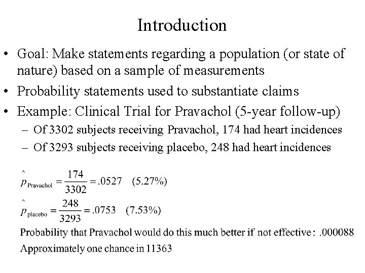
Introduction • Goal: Make statements regarding a population (or state of nature) based on a sample of measurements • Probability statements used to substantiate claims • Example: Clinical Trial for Pravachol (5 -year follow-up) – Of 3302 subjects receiving Pravachol, 174 had heart incidences – Of 3293 subjects receiving placebo, 248 had heart incidences

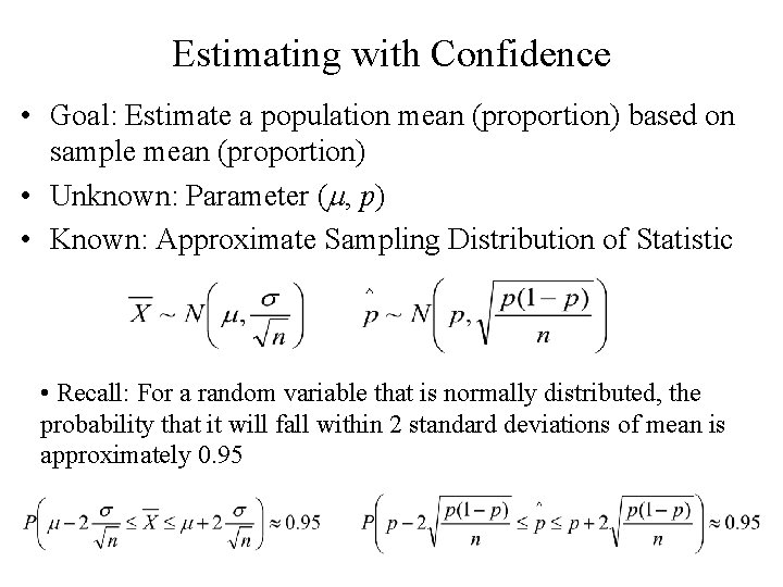
Estimating with Confidence • Goal: Estimate a population mean (proportion) based on sample mean (proportion) • Unknown: Parameter (m, p) • Known: Approximate Sampling Distribution of Statistic • Recall: For a random variable that is normally distributed, the probability that it will fall within 2 standard deviations of mean is approximately 0. 95

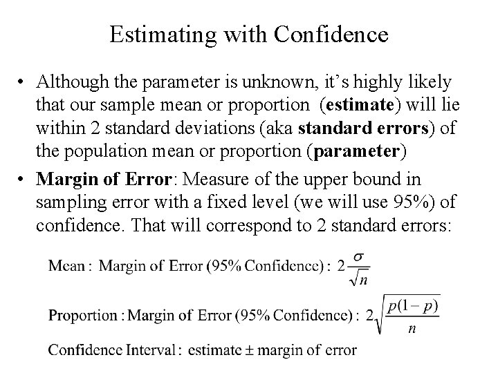
Estimating with Confidence • Although the parameter is unknown, it’s highly likely that our sample mean or proportion (estimate) will lie within 2 standard deviations (aka standard errors) of the population mean or proportion (parameter) • Margin of Error: Measure of the upper bound in sampling error with a fixed level (we will use 95%) of confidence. That will correspond to 2 standard errors:

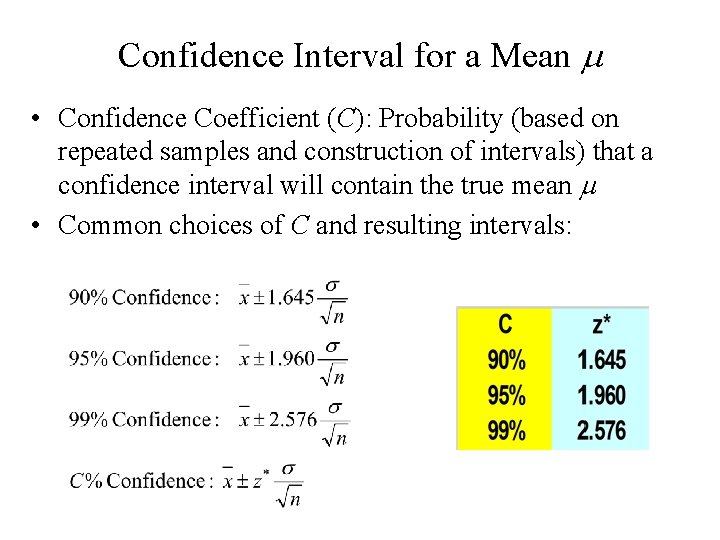
Confidence Interval for a Mean m • Confidence Coefficient (C): Probability (based on repeated samples and construction of intervals) that a confidence interval will contain the true mean m • Common choices of C and resulting intervals:

C m

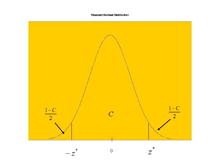
C 0

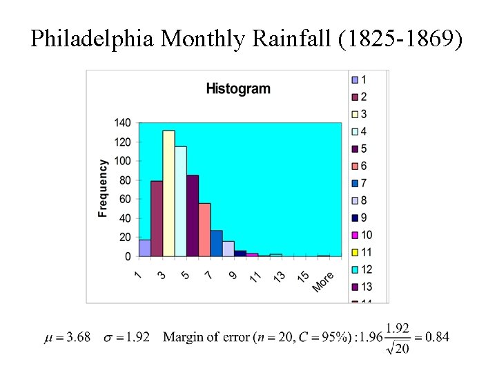
Philadelphia Monthly Rainfall (1825 -1869)

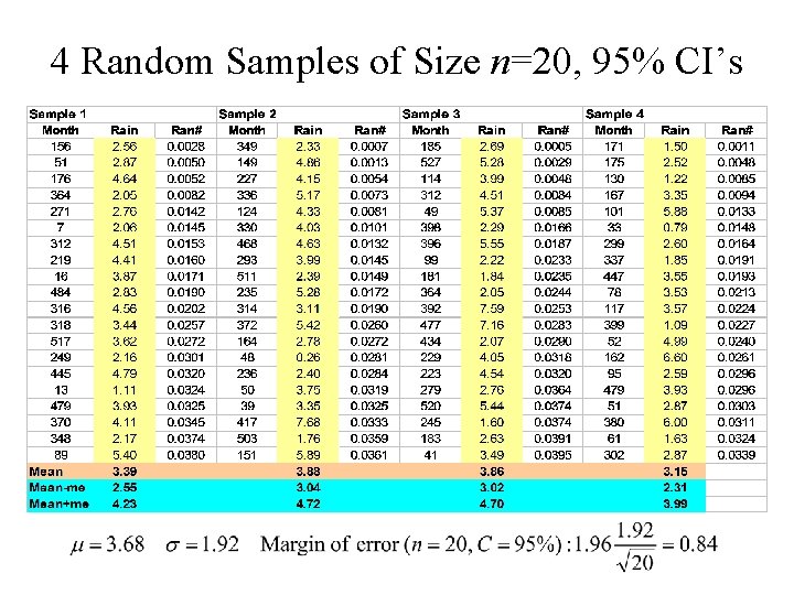
4 Random Samples of Size n=20, 95% CI’s

Factors Effecting Confidence Interval Width • Goal: Have precise (narrow) confidence intervals – Confidence Level (C): Increasing C implies increasing probability an interval contains parameter implies a wider confidence interval. Reducing C will shorten the interval (at a cost in confidence) – Sample size (n): Increasing n decreases standard error of estimate, margin of error, and width of interval (Quadrupling n cuts width in half) – Standard Deviation (s): More variable the individual measurements, the wider the interval. Potential ways to reduce s are to focus on more precise target population or use more precise measuring instrument. Often nothing can be done as nature determines s

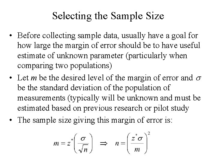
Selecting the Sample Size • Before collecting sample data, usually have a goal for how large the margin of error should be to have useful estimate of unknown parameter (particularly when comparing two populations) • Let m be the desired level of the margin of error and s be the standard deviation of the population of measurements (typically will be unknown and must be estimated based on previous research or pilot study • The sample size giving this margin of error is:

Precautions • Data should be simple random sample from population (or at least can be treated as independent observations) • More complex sampling designs have adjustments made to formulas (see Texts such as Elementary Survey Sampling by Scheaffer, Mendenhall, Ott) • Biased sampling designs give meaningless results • Small sample sizes from nonnormal distributions will have coverage probabilities (C) typically below the nominal level • Typically s is unknown. Replacing it with sample standard deviation s works as a good approximation in large samples

Significance Tests • Method of using sample (observed) data to challenge a hypothesis regarding a state of nature (represented as particular parameter value(s)) • Begin by stating a research hypothesis that challenges a statement of “status quo” (or equality of 2 populations) • State the current state or “status quo” as a statement regarding population parameter(s) • Obtain sample data and see to what extent it agrees/disagrees with the “status quo” • Conclude that the “status quo” is not true if observed data are highly unlikely (low probability) if it were true

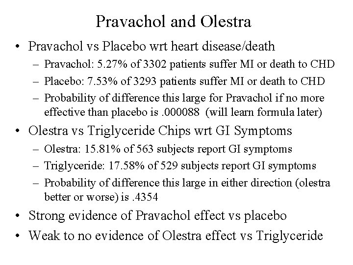
Pravachol and Olestra • Pravachol vs Placebo wrt heart disease/death – Pravachol: 5. 27% of 3302 patients suffer MI or death to CHD – Placebo: 7. 53% of 3293 patients suffer MI or death to CHD – Probability of difference this large for Pravachol if no more effective than placebo is. 000088 (will learn formula later) • Olestra vs Triglyceride Chips wrt GI Symptoms – Olestra: 15. 81% of 563 subjects report GI symptoms – Triglyceride: 17. 58% of 529 subjects report GI symptoms – Probability of difference this large in either direction (olestra better or worse) is. 4354 • Strong evidence of Pravachol effect vs placebo • Weak to no evidence of Olestra effect vs Triglyceride

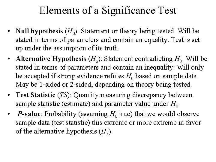
Elements of a Significance Test • Null hypothesis (H 0): Statement or theory being tested. Will be stated in terms of parameters and contain an equality. Test is set up under the assumption of its truth. • Alternative Hypothesis (Ha): Statement contradicting H 0. Will be stated in terms of parameters and contain an inequality. Will only be accepted if strong evidence refutes H 0 based on sample data. May be 1 -sided or 2 -sided, depending on theory being tested. • Test Statistic (TS): Quantity measuring discrepancy between sample statistic (estimate) and parameter value under H 0 • P-value: Probability (assuming H 0 true) that we would observe sample data (test statistic) this extreme or more extreme in favor of the alternative hypothesis (Ha)

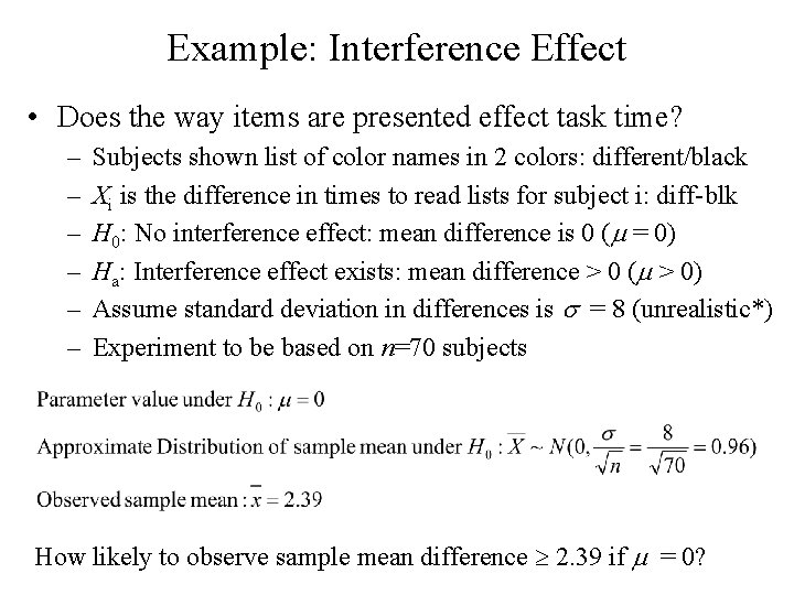
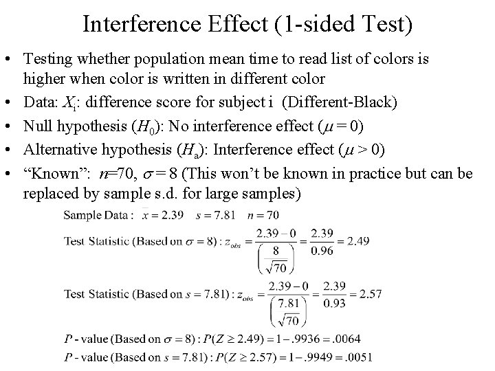
Example: Interference Effect • Does the way items are presented effect task time? – – – Subjects shown list of color names in 2 colors: different/black Xi is the difference in times to read lists for subject i: diff-blk H 0: No interference effect: mean difference is 0 (m = 0) Ha: Interference effect exists: mean difference > 0 (m > 0) Assume standard deviation in differences is s = 8 (unrealistic*) Experiment to be based on n=70 subjects How likely to observe sample mean difference 2. 39 if m = 0?

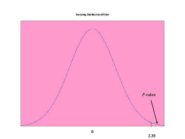
P-value 0 2. 39

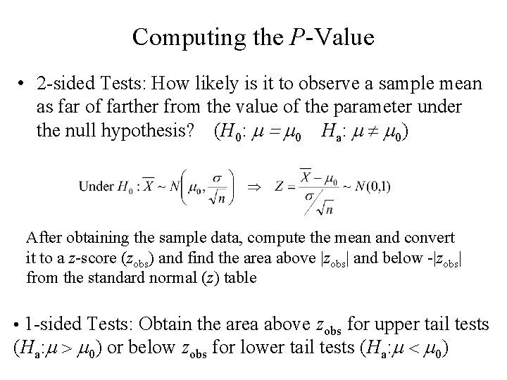
Computing the P-Value • 2 -sided Tests: How likely is it to observe a sample mean as far of farther from the value of the parameter under the null hypothesis? (H 0: m = m 0 Ha: m m 0) After obtaining the sample data, compute the mean and convert it to a z-score (zobs) and find the area above |zobs| and below -|zobs| from the standard normal (z) table • 1 -sided Tests: Obtain the area above zobs for upper tail tests (Ha: m > m 0) or below zobs for lower tail tests (Ha: m < m 0)

Interference Effect (1 -sided Test) • Testing whether population mean time to read list of colors is higher when color is written in different color • Data: Xi: difference score for subject i (Different-Black) • Null hypothesis (H 0): No interference effect (m = 0) • Alternative hypothesis (Ha): Interference effect (m > 0) • “Known”: n=70, s = 8 (This won’t be known in practice but can be replaced by sample s. d. for large samples)

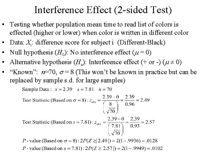
Interference Effect (2 -sided Test) • Testing whether population mean time to read list of colors is effected (higher or lower) when color is written in different color • Data: Xi: difference score for subject i (Different-Black) • Null hypothesis (H 0): No interference effect (m = 0) • Alternative hypothesis (Ha): Interference effect (+ or -) (m 0) • “Known”: n=70, s = 8 (This won’t be known in practice but can be replaced by sample s. d. for large samples)

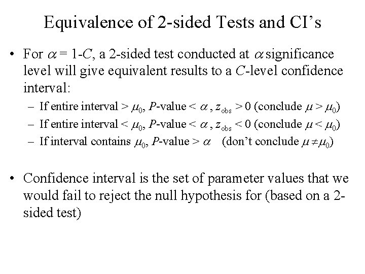
Equivalence of 2 -sided Tests and CI’s • For a = 1 -C, a 2 -sided test conducted at a significance level will give equivalent results to a C-level confidence interval: – If entire interval > m 0, P-value < a , zobs > 0 (conclude m > m 0) – If entire interval < m 0, P-value < a , zobs < 0 (conclude m < m 0) – If interval contains m 0, P-value > a (don’t conclude m m 0) • Confidence interval is the set of parameter values that we would fail to reject the null hypothesis for (based on a 2 sided test)

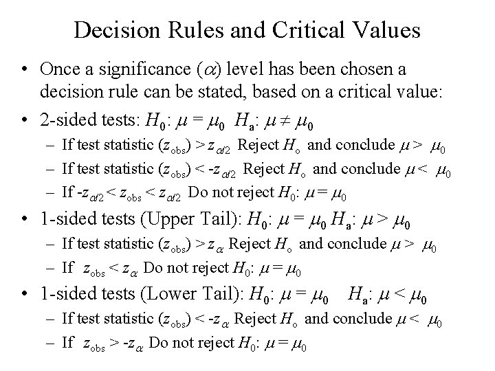
Decision Rules and Critical Values • Once a significance (a) level has been chosen a decision rule can be stated, based on a critical value: • 2 -sided tests: H 0: m = m 0 Ha: m m 0 – If test statistic (zobs) > za/2 Reject Ho and conclude m > m 0 – If test statistic (zobs) < -za/2 Reject Ho and conclude m < m 0 – If -za/2 < zobs < za/2 Do not reject H 0: m = m 0 • 1 -sided tests (Upper Tail): H 0: m = m 0 Ha: m > m 0 – If test statistic (zobs) > za Reject Ho and conclude m > m 0 – If zobs < za Do not reject H 0: m = m 0 • 1 -sided tests (Lower Tail): H 0: m = m 0 Ha: m < m 0 – If test statistic (zobs) < -za Reject Ho and conclude m < m 0 – If zobs > -za Do not reject H 0: m = m 0

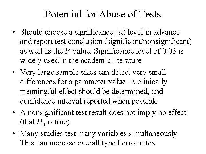
Potential for Abuse of Tests • Should choose a significance (a) level in advance and report test conclusion (significant/nonsignificant) as well as the P-value. Significance level of 0. 05 is widely used in the academic literature • Very large sample sizes can detect very small differences for a parameter value. A clinically meaningful effect should be determined, and confidence interval reported when possible • A nonsignificant test result does not imply no effect (that H 0 is true). • Many studies test many variables simultaneously. This can increase overall type I error rates

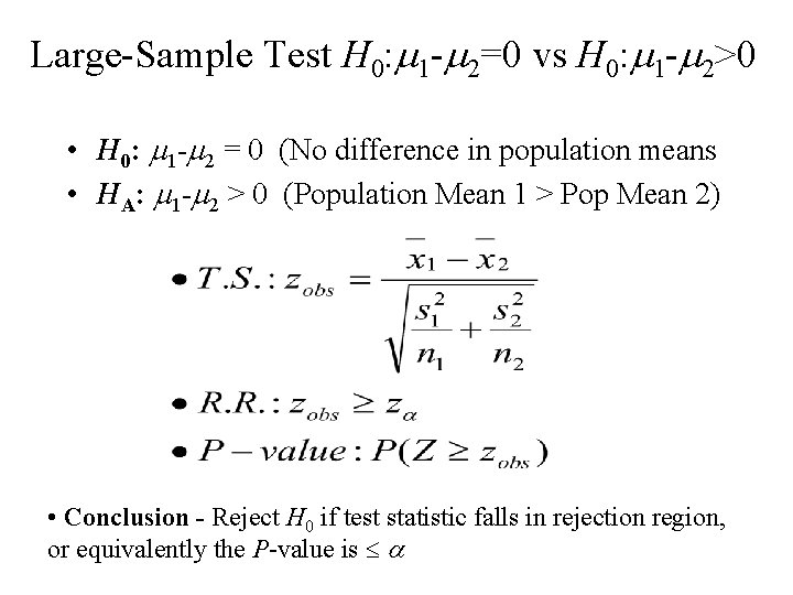
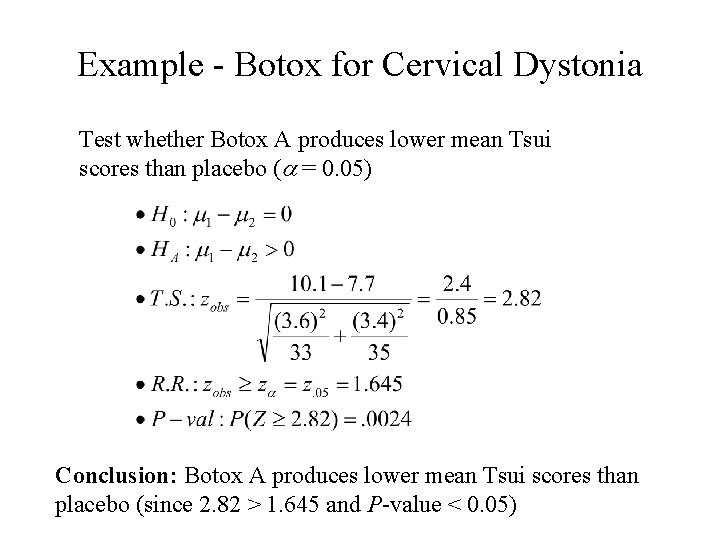
Large-Sample Test H 0: m 1 -m 2=0 vs H 0: m 1 -m 2>0 • H 0: m 1 -m 2 = 0 (No difference in population means • HA: m 1 -m 2 > 0 (Population Mean 1 > Pop Mean 2) • Conclusion - Reject H 0 if test statistic falls in rejection region, or equivalently the P-value is a

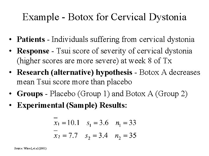
Example - Botox for Cervical Dystonia • Patients - Individuals suffering from cervical dystonia • Response - Tsui score of severity of cervical dystonia (higher scores are more severe) at week 8 of Tx • Research (alternative) hypothesis - Botox A decreases mean Tsui score more than placebo • Groups - Placebo (Group 1) and Botox A (Group 2) • Experimental (Sample) Results: Source: Wissel, et al (2001)

Example - Botox for Cervical Dystonia Test whether Botox A produces lower mean Tsui scores than placebo (a = 0. 05) Conclusion: Botox A produces lower mean Tsui scores than placebo (since 2. 82 > 1. 645 and P-value < 0. 05)

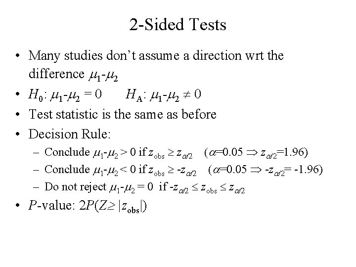
2 -Sided Tests • Many studies don’t assume a direction wrt the difference m 1 -m 2 • H 0: m 1 -m 2 = 0 HA: m 1 -m 2 0 • Test statistic is the same as before • Decision Rule: – Conclude m 1 -m 2 > 0 if zobs za/2 (a=0. 05 za/2=1. 96) – Conclude m 1 -m 2 < 0 if zobs -za/2 (a=0. 05 -za/2= -1. 96) – Do not reject m 1 -m 2 = 0 if -za/2 zobs za/2 • P-value: 2 P(Z |zobs|)

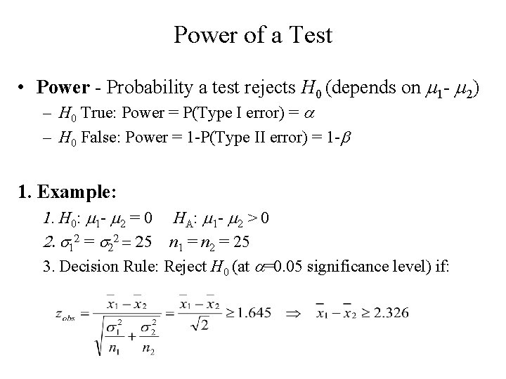
Power of a Test • Power - Probability a test rejects H 0 (depends on m 1 - m 2) – H 0 True: Power = P(Type I error) = a – H 0 False: Power = 1 -P(Type II error) = 1 -b 1. Example: 1. H 0: m 1 - m 2 = 0 HA: m 1 - m 2 > 0 2. s 12 = s 22 = 25 n 1 = n 2 = 25 3. Decision Rule: Reject H 0 (at a=0. 05 significance level) if:

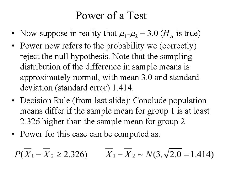
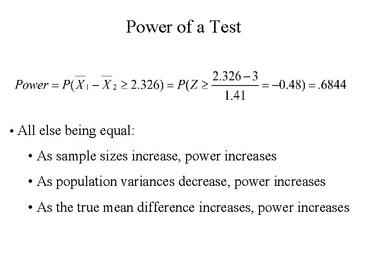
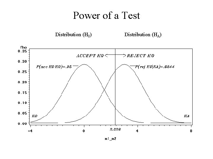
Power of a Test • Now suppose in reality that m 1 -m 2 = 3. 0 (HA is true) • Power now refers to the probability we (correctly) reject the null hypothesis. Note that the sampling distribution of the difference in sample means is approximately normal, with mean 3. 0 and standard deviation (standard error) 1. 414. • Decision Rule (from last slide): Conclude population means differ if the sample mean for group 1 is at least 2. 326 higher than the sample mean for group 2 • Power for this case can be computed as:

Power of a Test • All else being equal: • As sample sizes increase, power increases • As population variances decrease, power increases • As the true mean difference increases, power increases

Power of a Test Distribution (H 0) Distribution (HA)

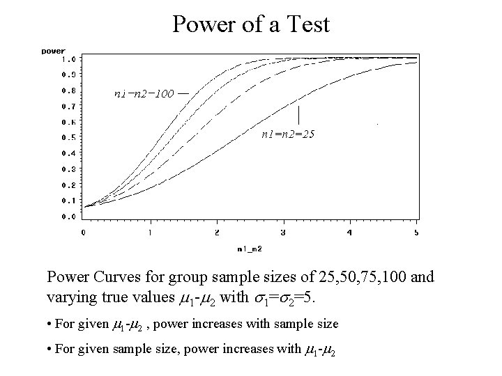
Power of a Test Power Curves for group sample sizes of 25, 50, 75, 100 and varying true values m 1 -m 2 with s 1=s 2=5. • For given m 1 -m 2 , power increases with sample size • For given sample size, power increases with m 1 -m 2

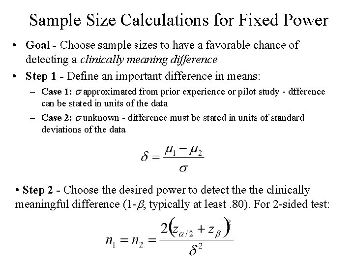
Sample Size Calculations for Fixed Power • Goal - Choose sample sizes to have a favorable chance of detecting a clinically meaning difference • Step 1 - Define an important difference in means: – Case 1: s approximated from prior experience or pilot study - dfference can be stated in units of the data – Case 2: s unknown - difference must be stated in units of standard deviations of the data • Step 2 - Choose the desired power to detect the clinically meaningful difference (1 -b, typically at least. 80). For 2 -sided test: