CHAPTER 6 Integration SECTION 6 1 Antiderivatives and

CHAPTER 6 Integration

SECTION 6. 1 Antiderivatives and Indefinite Integration

Definition of an Antiderivative A function F is an antiderivative of f on an interval I if F’(x) = f(x) for all x in I.

Theorem – Representation of Antiderivtives If F is an antiderivative of f on an interval I, then G is an antiderivative of f on the interval I if and only if G is on the form: G(x) = F(x) + C, for all x in I where C is a constant

Terminology C - is called the constant of integration G(x) = x 2 + c is the general solution of the differential equation G’(x) = 2 x Integration is the “inverse” of Differentiation

Differential Equation Is an equation that involves x, y and derivatives of y. EXAMPLES y’ = 3 x and y’ = x 2 + 1

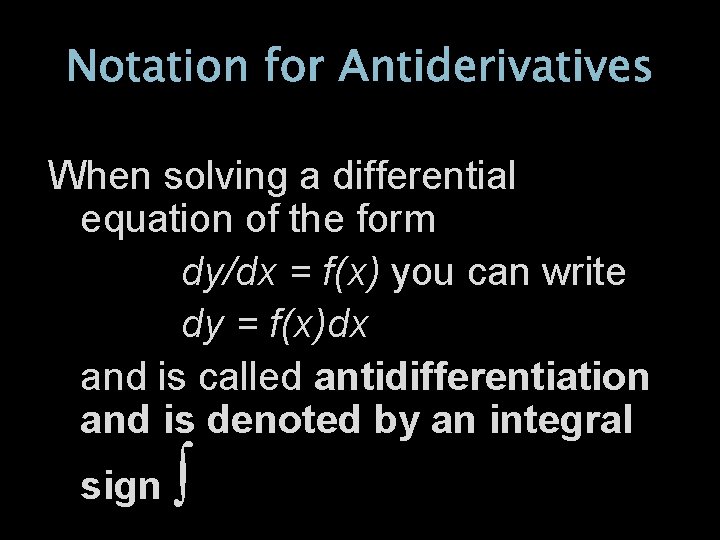
Notation for Antiderivatives When solving a differential equation of the form dy/dx = f(x) you can write dy = f(x)dx and is called antidifferentiation and is denoted by an integral sign ∫

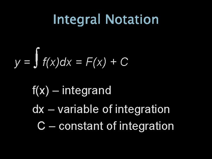
Integral Notation y= ∫ f(x)dx = F(x) + C f(x) – integrand dx – variable of integration C – constant of integration

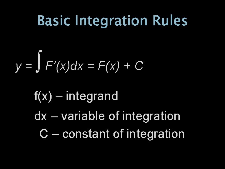
Basic Integration Rules y= ∫ F’(x)dx = F(x) + C f(x) – integrand dx – variable of integration C – constant of integration

Basic Integration Rules DIFFERENTIATION FORMULA � � � d/dx [c] = 0 d/dx [kx] = k d/dx [kf(x)] = kf’(x) d/dx [f(x) ± g(x)] = f’(x) ± g’(x) d/dx [xn] = nxn-1 INTEGRATION FORMULA � � � ∫ 0 dx = c ∫ kdx = kx + c ∫ kf(x)dx = k ∫ f(x) dx ∫ f(x) ± g(x)]dx = ∫ f(x) dx ± ∫ g(x) dx ∫ xn dx = (xn+1)/(n+1) + c, n≠ - 1 (Power Rule)

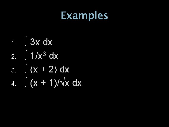
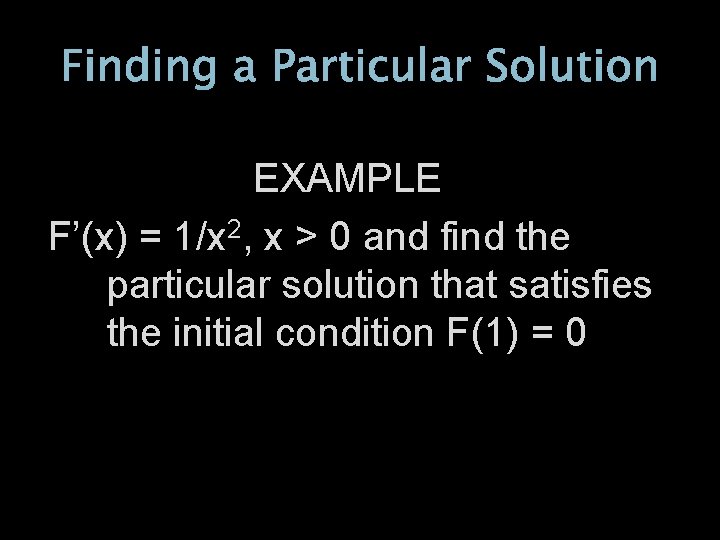
Examples 1. 2. 3. 4. ∫ 3 x dx ∫ 1/x 3 dx ∫ (x + 2) dx ∫ (x + 1)/√x dx

Finding a Particular Solution EXAMPLE F’(x) = 1/x 2, x > 0 and find the particular solution that satisfies the initial condition F(1) = 0

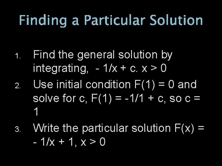
Finding a Particular Solution 1. 2. 3. Find the general solution by integrating, - 1/x + c. x > 0 Use initial condition F(1) = 0 and solve for c, F(1) = -1/1 + c, so c = 1 Write the particular solution F(x) = - 1/x + 1, x > 0

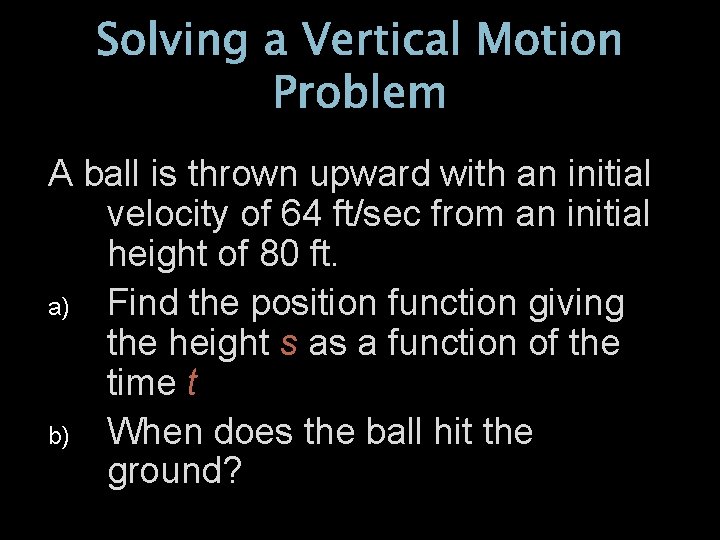
Solving a Vertical Motion Problem A ball is thrown upward with an initial velocity of 64 ft/sec from an initial height of 80 ft. a) Find the position function giving the height s as a function of the time t b) When does the ball hit the ground?

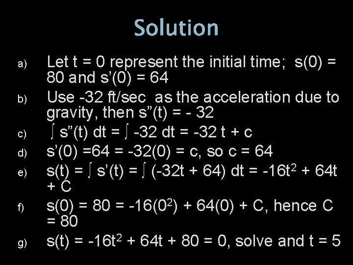
Solution a) b) c) d) e) f) g) Let t = 0 represent the initial time; s(0) = 80 and s’(0) = 64 Use -32 ft/sec as the acceleration due to gravity, then s”(t) = - 32 ∫ s”(t) dt = ∫ -32 dt = -32 t + c s’(0) =64 = -32(0) = c, so c = 64 s(t) = ∫ s’(t) = ∫ (-32 t + 64) dt = -16 t 2 + 64 t +C s(0) = 80 = -16(02) + 64(0) + C, hence C = 80 s(t) = -16 t 2 + 64 t + 80 = 0, solve and t = 5

SECTION 6. 2 Area

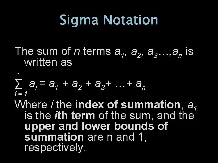
Sigma Notation The sum of n terms a 1, a 2, a 3…, an is written as n ∑ ai = a 1 + a 2 + a 3+ …+ an i=1 Where i the index of summation, a 1 is the ith term of the sum, and the upper and lower bounds of summation are n and 1, respectively.

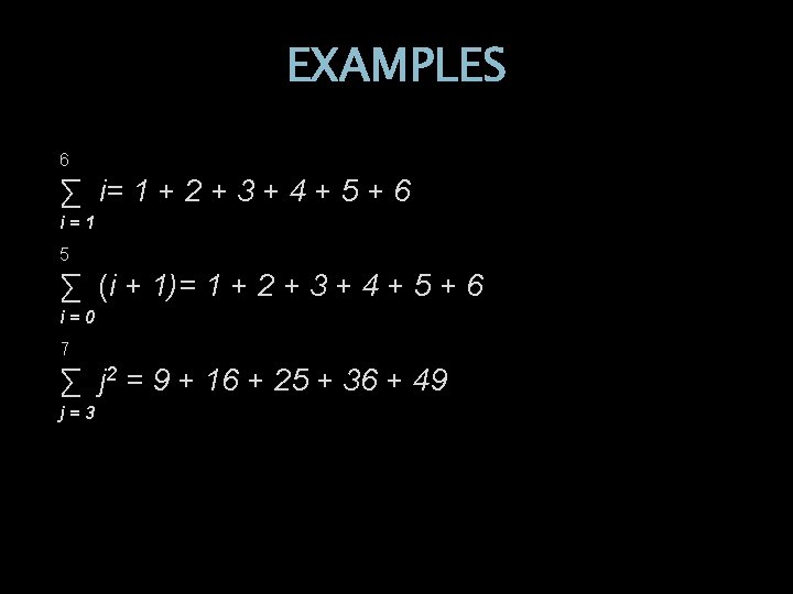
EXAMPLES 6 ∑ i= 1 + 2 + 3 + 4 + 5 + 6 i=1 5 ∑ (i + 1)= 1 + 2 + 3 + 4 + 5 + 6 i=0 7 ∑ j 2 = 9 + 16 + 25 + 36 + 49 j=3

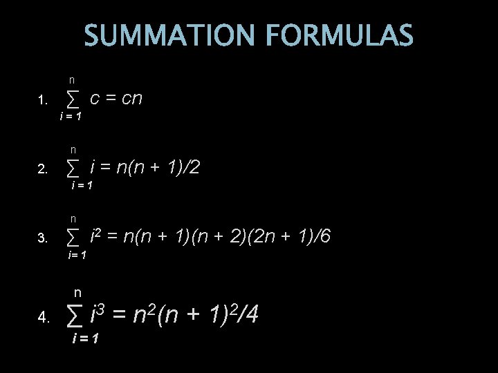
SUMMATION FORMULAS n 1. ∑ c = cn i=1 n 2. ∑ i = n(n + 1)/2 i=1 n 3. ∑ i 2 = n(n + 1)(n + 2)(2 n + 1)/6 i= 1 n 4. ∑ i 3 = n 2(n + 1)2/4 i=1

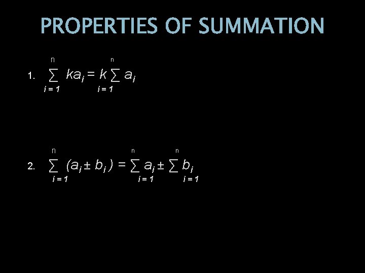
PROPERTIES OF SUMMATION n 1. ∑ kai = k ∑ ai i=1 n 2. n i=1 n n ∑ (ai ± bi ) = ∑ ai ± ∑ bi i=1 i=1

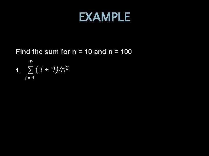
EXAMPLE Find the sum for n = 10 and n = 100 n 1. ∑ ( i + 1)/n 2 i=1

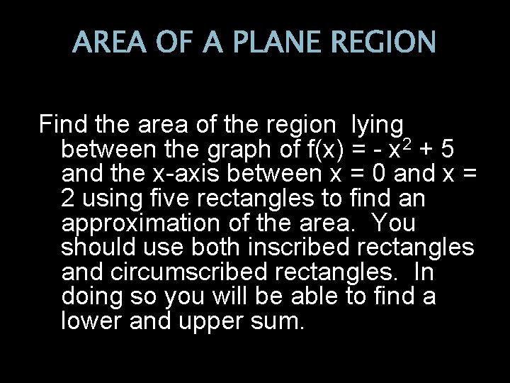
AREA OF A PLANE REGION Find the area of the region lying between the graph of f(x) = - x 2 + 5 and the x-axis between x = 0 and x = 2 using five rectangles to find an approximation of the area. You should use both inscribed rectangles and circumscribed rectangles. In doing so you will be able to find a lower and upper sum.

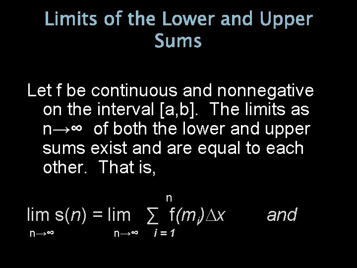
Limits of the Lower and Upper Sums Let f be continuous and nonnegative on the interval [a, b]. The limits as n→∞ of both the lower and upper sums exist and are equal to each other. That is, n lim s(n) = lim ∑ f(mi) x n→∞ i=1 and

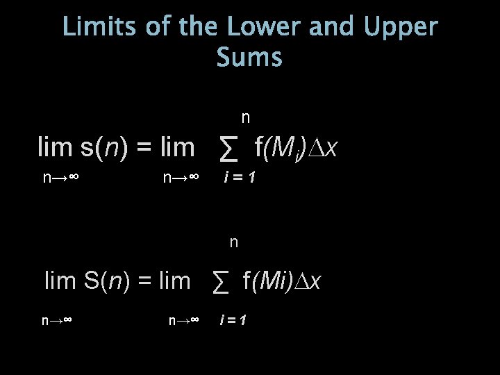
Limits of the Lower and Upper Sums n lim s(n) = lim ∑ f(Mi) x n→∞ i=1 n lim S(n) = lim ∑ f(Mi) x n→∞ i=1

Definition of the Area of a Region in the Plane Let f be continuous and nonnegative on the interval [a, b]. The area of the region bounded by the graph of f, the x-axis, and the vertical lines x= a and x = b is n Area = lim ∑ f(ci) x, xi -1 ci xi n→∞ i=1 Where x = (b-a)/n

EXAMPLE Fine the area of the region bounded by the graph of f(x) =x 3, the x-axis, and the vertical lines x=0 and x =1. 1. Partition the interval [0, 1] into n subintervals each of width 1/n = x 2. Simplify using the formula below and A = 1/4 n Area = lim ∑ f(ci) x, xi -1 ci xi n→∞ i=1 Where x = (b-a)/n

SECTION 6. 3 Riemann Sums and Definite Integrals

Definition of Riemann Sum Let f be defined on the closed interval [a, b] and let be a partition of [a, b] given by a = xo < x 1 < x 2 < …<xn-1<xn =b Where xi is the width of the ith subinterval. If ci is any point in the ith subinterval, then the sum n f(ci) xi , xi-1 ci xi is called a Riemann i =1 sum of f for the partition

Definition of the Norm The width of the largest subinterval of a partition is the norm of the partition and is denoted by . If every subinterval is of equal width, the partition is regular and the norm is denoted by = x = (b – a)/n

Definite Integrals If f is defined on the closed interval [a, b] and the limit n lim ∑ f(ci) x → 0 i=1 exists, then f is integrable on [a, b] and the limit is b ∫ f(x) dx a The number a is the lower limit of integration, and the number b is the upper limit of integration

Continuity Implies Integrability If a function f is continuous on the closed interval [a, b], then f is integrable on ]a, b]

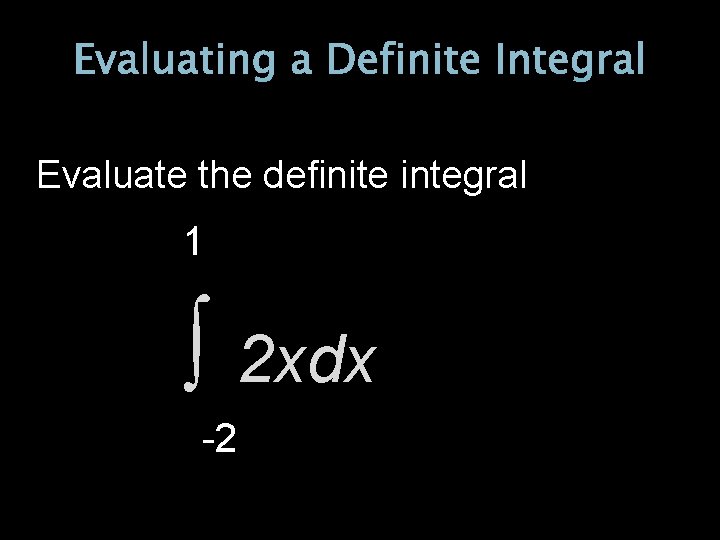
Evaluating a Definite Integral Evaluate the definite integral 1 ∫ 2 xdx -2

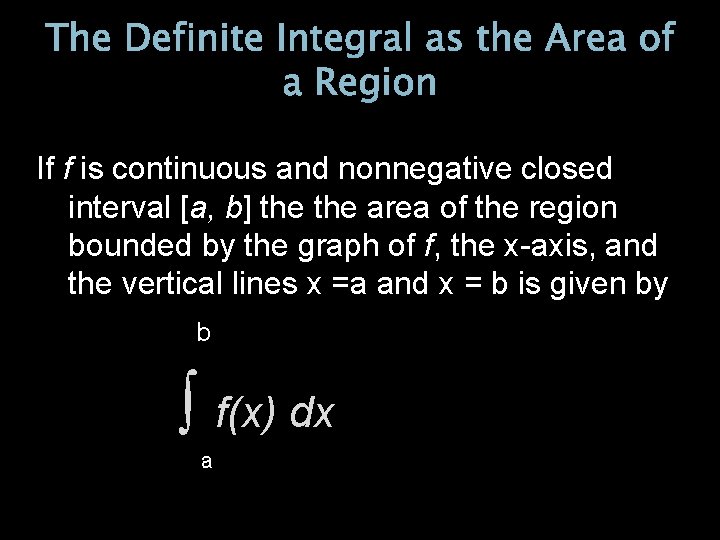
The Definite Integral as the Area of a Region If f is continuous and nonnegative closed interval [a, b] the area of the region bounded by the graph of f, the x-axis, and the vertical lines x =a and x = b is given by b ∫ f(x) dx a

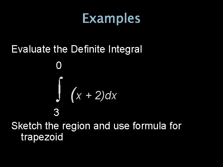
Examples Evaluate the Definite Integral 0 ∫ (x + 2)dx 3 Sketch the region and use formula for trapezoid

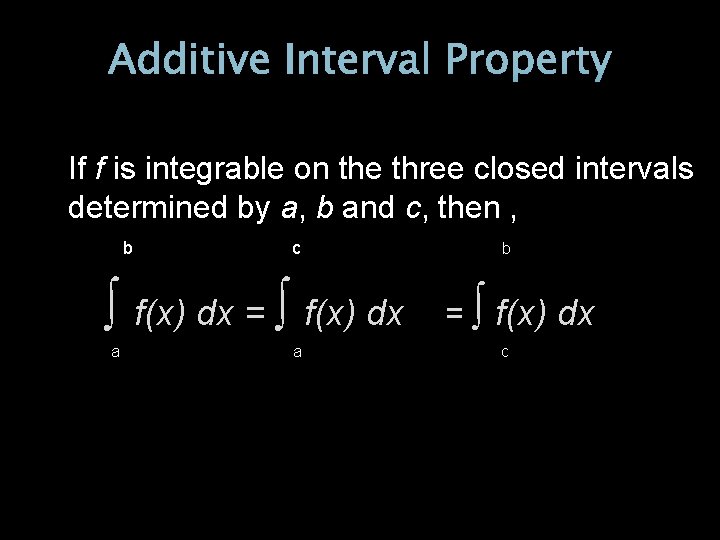
Additive Interval Property If f is integrable on the three closed intervals determined by a, b and c, then , b c ∫ f(x) dx = ∫ f(x) dx a a b = ∫ f(x) dx c

Properties of Definite Integrals If f and g are integrable on [a, b] and k is a constant, then the functions of kf and f ± g are integrable on [a, b], and b 1. b ∫kf dx = k ∫ f(x) dx a a

Properties of Definite Integrals If f and g are integrable on [a, b] and k is a constant, then the functions of kf and f ± g are integrable on [a, b], and b 1. b b ∫[f(x) ± g(x)] dx = ∫ f(x) dx ± ∫ f(x) dx a a a

SECTION 6. 4 THE FUNDAMENTAL THEOREM OF CALCULUS

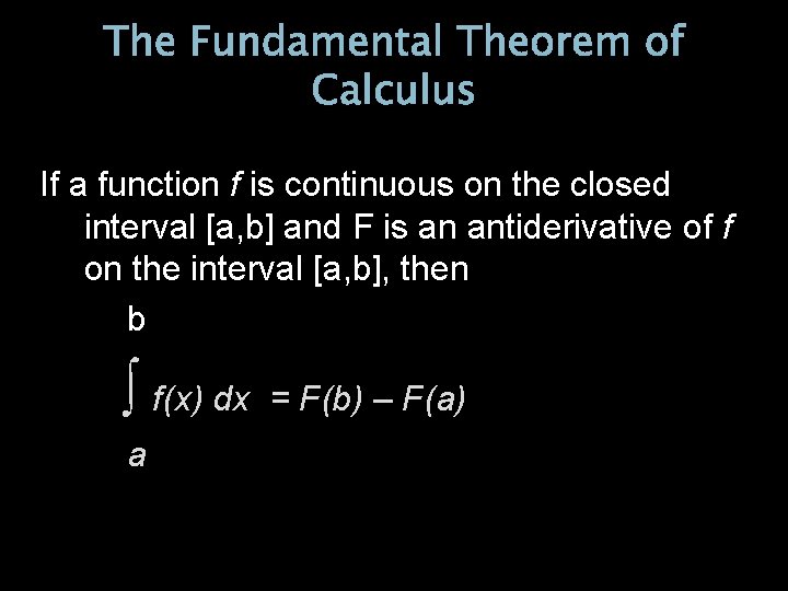
The Fundamental Theorem of Calculus If a function f is continuous on the closed interval [a, b] and F is an antiderivative of f on the interval [a, b], then b ∫ f(x) dx a = F(b) – F(a)

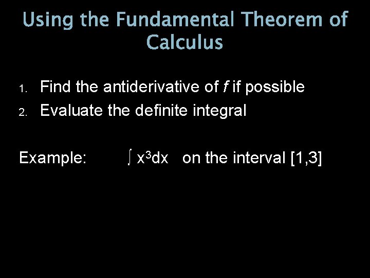
Using the Fundamental Theorem of Calculus 1. 2. Find the antiderivative of f if possible Evaluate the definite integral Example: ∫ x 3 dx on the interval [1, 3]

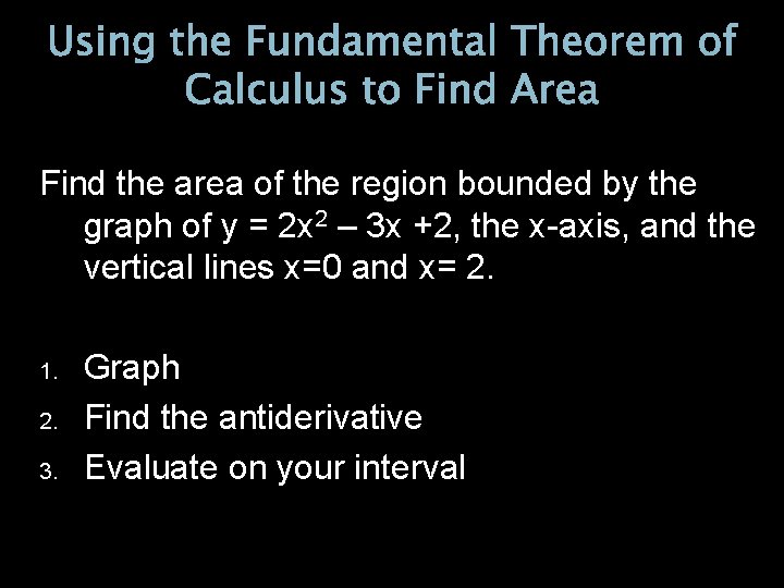
Using the Fundamental Theorem of Calculus to Find Area Find the area of the region bounded by the graph of y = 2 x 2 – 3 x +2, the x-axis, and the vertical lines x=0 and x= 2. 1. 2. 3. Graph Find the antiderivative Evaluate on your interval

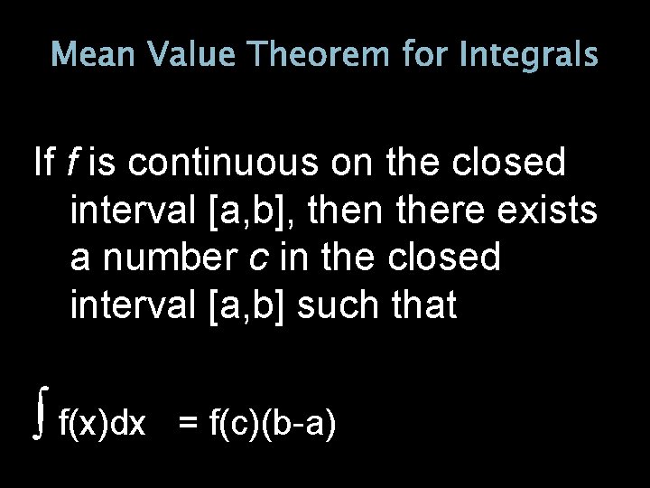
Mean Value Theorem for Integrals If f is continuous on the closed interval [a, b], then there exists a number c in the closed interval [a, b] such that ∫ f(x)dx = f(c)(b-a)

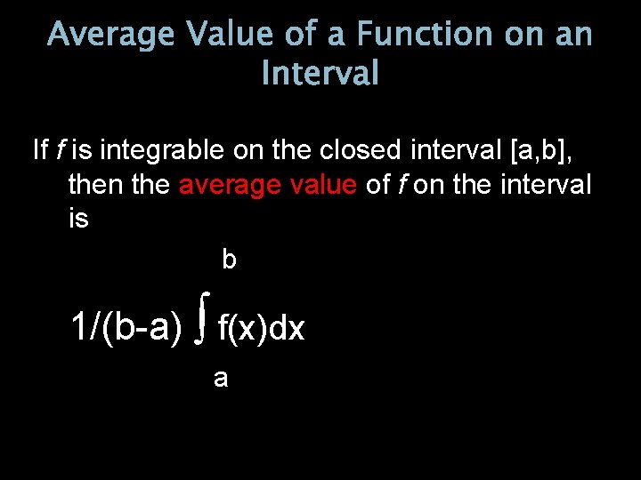
Average Value of a Function on an Interval If f is integrable on the closed interval [a, b], then the average value of f on the interval is b 1/(b-a) ∫ f(x)dx a

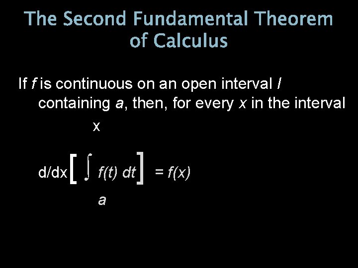
The Second Fundamental Theorem of Calculus If f is continuous on an open interval I containing a, then, for every x in the interval x d/dx [ ∫ f(t) dt] = f(x) a

SECTION 6. 5 INTEGRATION BY SUBSTITUTION

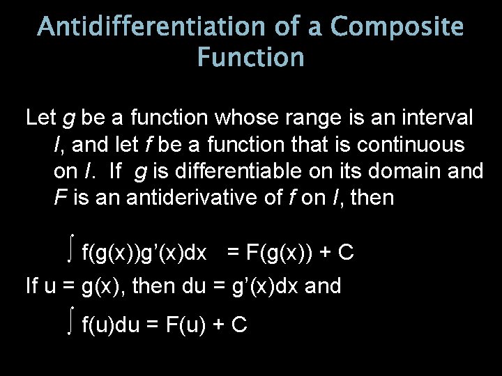
Antidifferentiation of a Composite Function Let g be a function whose range is an interval I, and let f be a function that is continuous on I. If g is differentiable on its domain and F is an antiderivative of f on I, then ∫ f(g(x))g’(x)dx = F(g(x)) + C If u = g(x), then du = g’(x)dx and ∫ f(u)du = F(u) + C

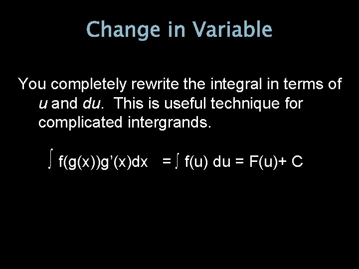
Change in Variable You completely rewrite the integral in terms of u and du. This is useful technique for complicated intergrands. ∫ f(g(x))g’(x)dx = ∫ f(u) du = F(u)+ C

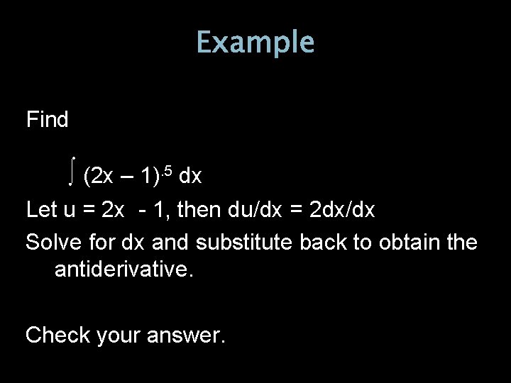
Example Find ∫ (2 x – 1). 5 dx Let u = 2 x - 1, then du/dx = 2 dx/dx Solve for dx and substitute back to obtain the antiderivative. Check your answer.

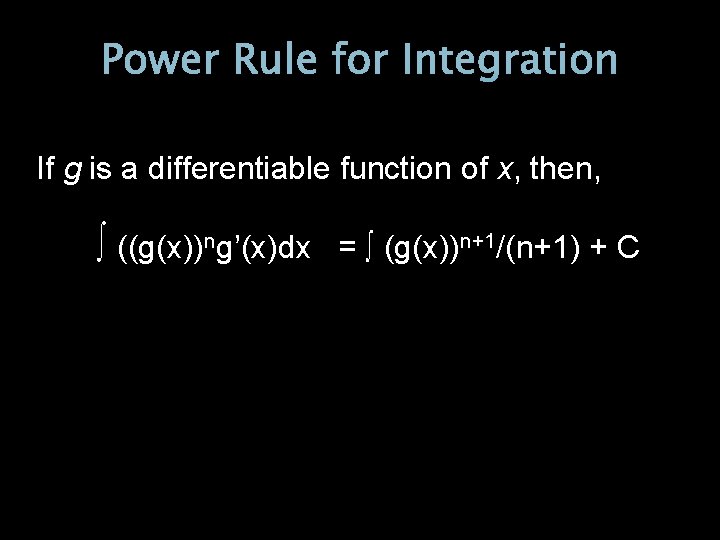
Power Rule for Integration If g is a differentiable function of x, then, ∫ ((g(x))ng’(x)dx = ∫ (g(x))n+1/(n+1) + C

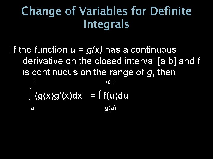
Change of Variables for Definite Integrals If the function u = g(x) has a continuous derivative on the closed interval [a, b] and f is continuous on the range of g, then, b ∫ (g(x)g’(x)dx a g(b) = ∫ f(u)du g(a)

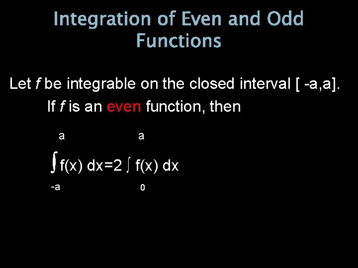
Integration of Even and Odd Functions Let f be integrable on the closed interval [ -a, a]. If f is an even function, then a a ∫ f(x) dx=2 ∫ f(x) dx -a 0

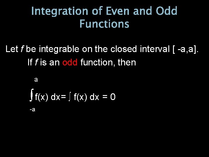
Integration of Even and Odd Functions Let f be integrable on the closed interval [ -a, a]. If f is an odd function, then a ∫ f(x) dx= ∫ f(x) dx = 0 -a

SECTION 6. 6 NUMERICAL INTEGRATION

Trapezoidal Rule Let f be continuous on [a, b]. The trapezoidal Rule for approximating ∫ f(x) dx (b-a)/2 n [f(x 0) = 2(f(x 1) +…. . +2 f(xn-1) + f(xn)]

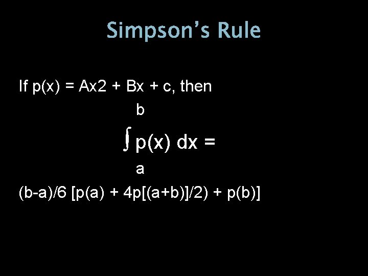
Simpson’s Rule If p(x) = Ax 2 + Bx + c, then b ∫ p(x) dx = a (b-a)/6 [p(a) + 4 p[(a+b)]/2) + p(b)]

END