Chapter 6 Human Capital Mc GrawHillIrwin Copyright 2010

Chapter 6 Human Capital Mc. Graw-Hill/Irwin Copyright © 2010 by The Mc. Graw-Hill Companies, Inc. All rights reserved.

Introduction • People bring into the labor market a unique set of abilities and acquired skills known as human capital. • Workers add to their stock of human capital throughout their lives, especially via work experience and education. 6 -2

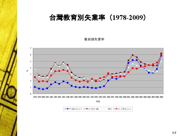
Education: Stylized Facts • Education is strongly correlated with: – Labor force participation rates – Unemployment rates – Earnings 6 -3

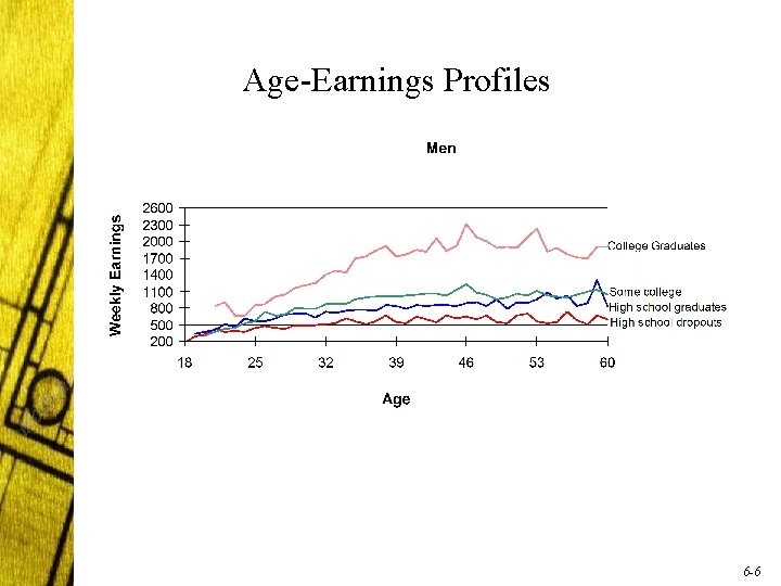
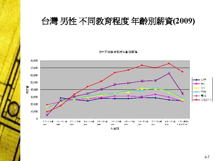
Age-Earnings Profiles 6 -6

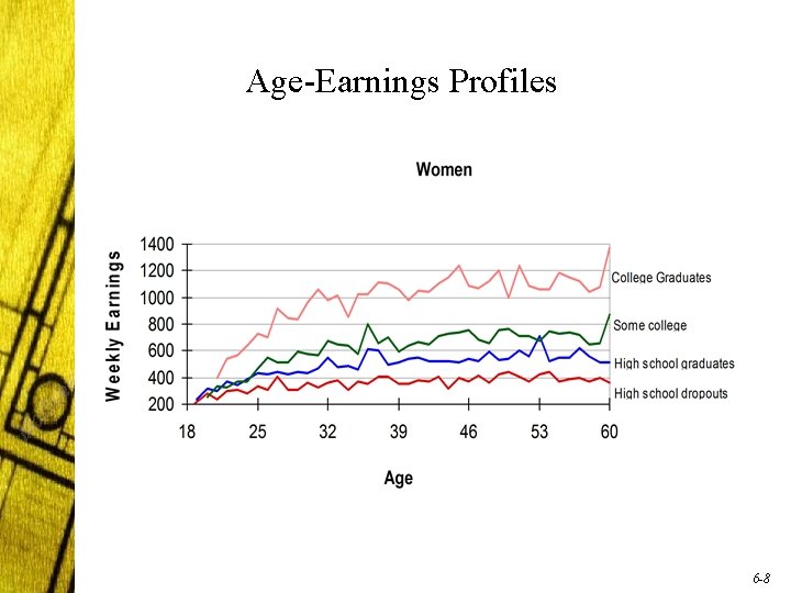
Age-Earnings Profiles 6 -8

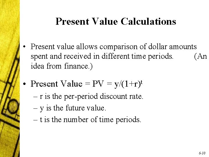
Present Value Calculations • Present value allows comparison of dollar amounts spent and received in different time periods. (An idea from finance. ) • Present Value = PV = y/(1+r)t – r is the per-period discount rate. – y is the future value. – t is the number of time periods. 6 -10

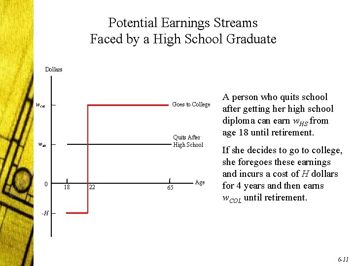
Potential Earnings Streams Faced by a High School Graduate Dollars Goes to College w. COL Quits After High School w. HS 0 18 22 65 Age A person who quits school after getting her high school diploma can earn w. HS from age 18 until retirement. If she decides to go to college, she foregoes these earnings and incurs a cost of H dollars for 4 years and then earns w. COL until retirement. -H 6 -11

The Schooling Model • Real earnings (earnings adjusted for inflation). • Age-earnings profile: the wage profile over a worker’s lifespan. • The higher the discount rate, the less likely someone will invest in education (since they are less future oriented). • The discount rate depends on: – the market rate of interest. – time preferences: how a person feels about giving up today’s consumption in return for future rewards. 6 -12

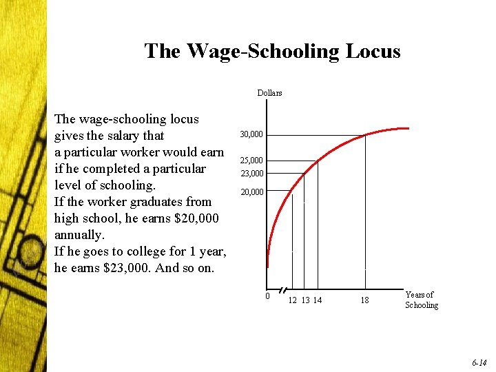
The Wage-Schooling Locus • The salaries firms are willing to pay workers depends on the level of schooling. • Properties of the wage-schooling locus. – The wage-schooling locus is upward sloping. – The wage-schooling locus is concave, reflecting diminishing returns to schooling. 6 -13

The Wage-Schooling Locus Dollars The wage-schooling locus gives the salary that a particular worker would earn if he completed a particular level of schooling. If the worker graduates from high school, he earns $20, 000 annually. If he goes to college for 1 year, he earns $23, 000. And so on. 30, 000 25, 000 23, 000 20, 000 0 12 13 14 18 Years of Schooling 6 -14

Education and the Wage Gap • Observed data on earnings and schooling does not allow us to estimate returns to schooling. • In theory, a more able person gets more from an additional year of education. • Ability bias: The extent to which unobserved ability differences exist affects estimates on returns to schooling, since the ability difference may be the true source of the wage differential. 6 -15

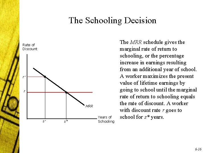
The Schooling Decision Rate of Discount r r MRR s s* Years of Schooling The MRR schedule gives the marginal rate of return to schooling, or the percentage increase in earnings resulting from an additional year of school. A worker maximizes the present value of lifetime earnings by going to school until the marginal rate of return to schooling equals the rate of discount. A worker with discount rate r goes to school for s* years. 6 -16

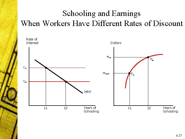
Schooling and Earnings When Workers Have Different Rates of Discount Rate of Interest Dollars w. HS PBO r. AL w. DROP PAL r. BO MRR 11 12 Years of Schooling 6 -17

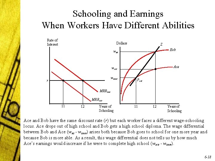
Schooling and Earnings When Workers Have Different Abilities Rate of Interest Dollars Z Bob w. HS Ace w. ACE w. DROP r PACE MRRBOB MRRACE 11 12 Years of Schooling Ace and Bob have the same discount rate (r) but each worker faces a different wage-schooling locus. Ace drops out of high school and Bob gets a high school diploma. The wage differential between Bob and Ace (w. HS - w. DROP) arises both because Bob goes to school for one more year and because Bob is more able. As a result, this wage differential does not tells us by how much Ace’s earnings would increase if he were to complete high school (w. ACE - w. DROP). 6 -18

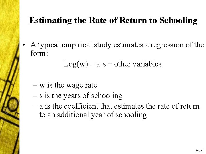
Estimating the Rate of Return to Schooling • A typical empirical study estimates a regression of the form: Log(w) = a·s + other variables – w is the wage rate – s is the years of schooling – a is the coefficient that estimates the rate of return to an additional year of schooling 6 -19

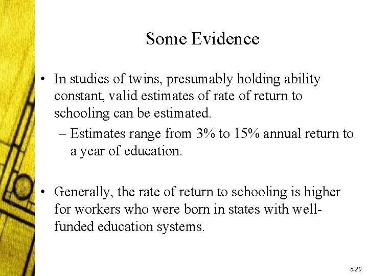
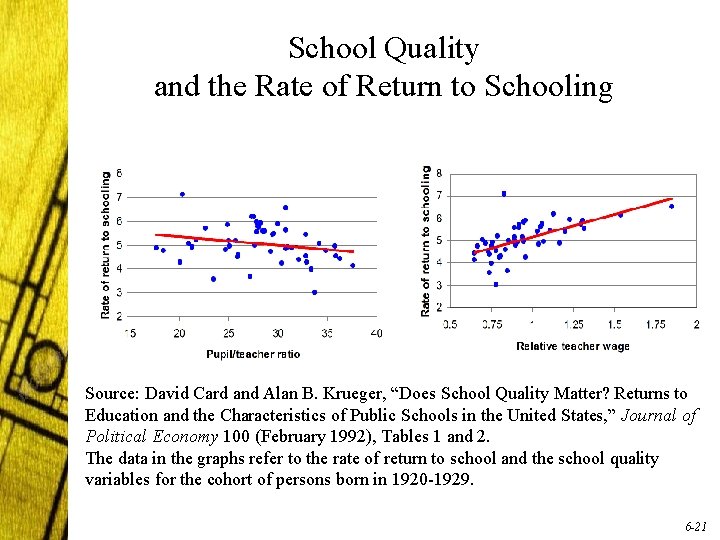
Some Evidence • In studies of twins, presumably holding ability constant, valid estimates of rate of return to schooling can be estimated. – Estimates range from 3% to 15% annual return to a year of education. • Generally, the rate of return to schooling is higher for workers who were born in states with wellfunded education systems. 6 -20

School Quality and the Rate of Return to Schooling Source: David Card and Alan B. Krueger, “Does School Quality Matter? Returns to Education and the Characteristics of Public Schools in the United States, ” Journal of Political Economy 100 (February 1992), Tables 1 and 2. The data in the graphs refer to the rate of return to school and the school quality variables for the cohort of persons born in 1920 -1929. 6 -21

Do Workers Maximize Lifetime Earnings? • The schooling model workers select their level of education present value of lifetime earnings. assumes that to maximize the – once a choice is made, we cannot observe the earnings associated with the non-choice. • Workers may select themselves into jobs for which they are better suited. • Self-Selection Bias 6 -22

Schooling as a Signal • Education reveals a level of attainment which signals a worker’s qualifications or innate ability to potential employers. • Information that is used to allocate workers in the labor market is called a signal. • There could be a “separating equilibrium. ” – Low-productivity workers choose not to obtain X years of education, voluntarily signaling their low productivity. – High-productivity workers choose to get at least X years of schooling and separate themselves from the pack. 6 -23

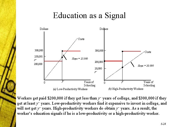
Education as a Signal Dollars Costs 300, 000 250, 001 y Costs Slope = 25, 000 200, 000 Slope = 20, 000 y Years of Schooling (a) Low-Productivity Workers 0 y Years of Schooling (b) High-Productivity Workers get paid $200, 000 if they get less than y years of college, and $300, 000 if they get at least y years. Low-productivity workers find it expensive to invest in college, and will not get y years. High-productivity workers do obtain y years. As a result, the worker’s education signals if he is a low-productivity or a high-productivity worker. 6 -24

Implications of Schooling as a Signal • Education is more than a signal, it alters the stock of human capital. • Social return to schooling (percentage increase in national income) is likely to be positive even if a particular worker’s human capital is not increased. 6 -25

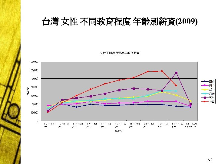
Post-School Human Capital Investments • Three important properties of age-earnings profiles: – Highly educated workers earn more than less educated workers. – Earnings rise over time at a decreasing rate. – The age-earnings profiles of different education cohorts diverge over time (they “fan outwards”). – Earnings increase faster for more educated workers. 6 -26

On-The-Job Training • Most workers augment their human capital stock through on-the-job training (OJT) after completing education investments. • Two types of OJT: – General: training that is useful at all firms once it is acquired. – Specific: training that is useful only at the firm where it is acquired. 6 -27

Implications • Firms only provide general training if they do not pay the costs. • In order for the firm to willingly pay some of the costs of specific training, the firm must share in the returns to specific training. Engaging in specific training eliminates the possibility of the worker separating from the job in the post-training period. 6 -28

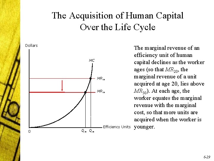
The Acquisition of Human Capital Over the Life Cycle Dollars MC MR 20 MR 30 0 Q 30 Q 20 Efficiency Units The marginal revenue of an efficiency unit of human capital declines as the worker ages (so that MR 20, the marginal revenue of a unit acquired at age 20, lies above MR 30). At each age, the worker equates the marginal revenue with the marginal cost, so that more units are acquired when the worker is younger. 6 -29

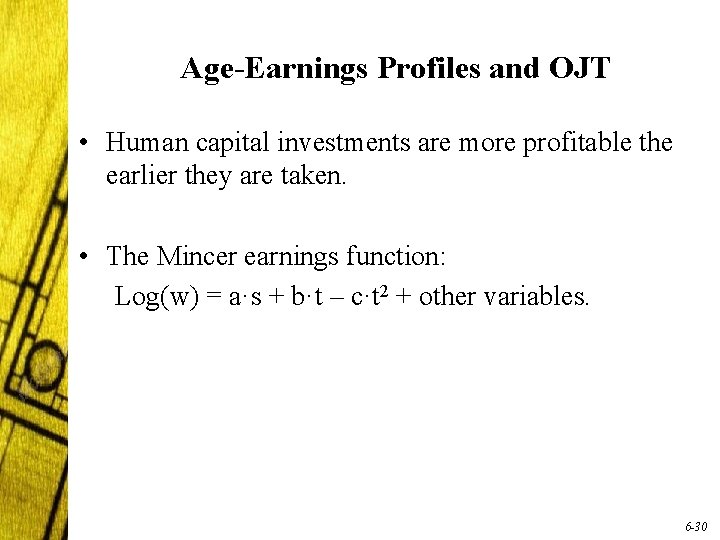
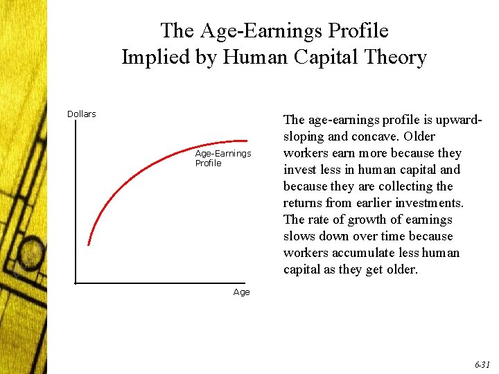
Age-Earnings Profiles and OJT • Human capital investments are more profitable the earlier they are taken. • The Mincer earnings function: Log(w) = a·s + b·t – c·t 2 + other variables. 6 -30

The Age-Earnings Profile Implied by Human Capital Theory Dollars Age-Earnings Profile The age-earnings profile is upwardsloping and concave. Older workers earn more because they invest less in human capital and because they are collecting the returns from earlier investments. The rate of growth of earnings slows down over time because workers accumulate less human capital as they get older. Age 6 -31

Policy Application: Evaluating Government Training Programs • Aimed at exposing disadvantaged and low-income workers to training programs. • $4 billion of federal spending per year. • Studies of the return to these human capital investments are unclear, largely because of selfselection bias. 6 -32

Social Experiments • National Supported Worker Demonstration (NSW). – Results of the NSW suggest a 10% return to investments in human capital for workers treated under the program. 6 -33