Chapter 6 Explanatory Models 2 TimeSeries Decomposition 2019

Chapter 6 Explanatory Models 2: Time-Series Decomposition © 2019 Mc. Graw-Hill Education. All rights reserved. Authorized only for instructor use in the classroom. No reproduction or further distribution permitted without the prior written consent of Mc. Graw-Hill Education.

Explanatory Models 2. Time-Series Decomposition(Chapter 6) The information provided by time-series decomposition is consistent with the way managers tend to look at data. © 2019 Mc. Graw-Hill Education.

Time Series Decomposition 1 This is the classical approach to economic forecasting. It assumes that an economic time series can be into four components: 1. secular trend 2. seasonal variation 3. cyclical variation © 2019 Mc. Graw-Hill Education.

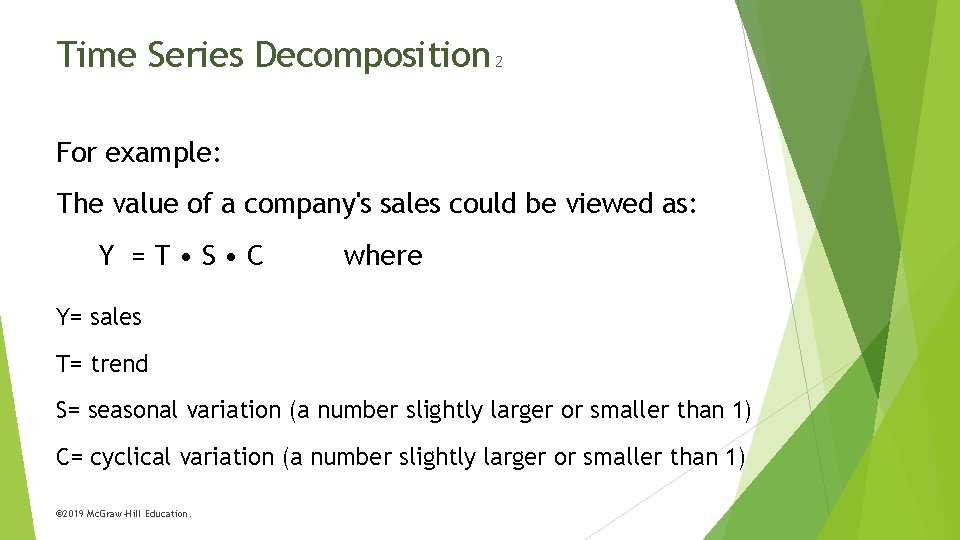
Time Series Decomposition 2 For example: The value of a company's sales could be viewed as: Y =T • S • C where Y= sales T= trend S= seasonal variation (a number slightly larger or smaller than 1) C= cyclical variation (a number slightly larger or smaller than 1) © 2019 Mc. Graw-Hill Education.

Decomposing a Series 1 Trend: a trend is a relatively smooth long-term movement of a time series. Seasonal variation: In a particular month, the value of an economic variable is likely to differ from what would be expected on the basis of its trend, because of seasonal factors. © 2019 Mc. Graw-Hill Education.

Decomposing a Series 2 Cyclical variation: another reason why an economic variable may differ from its trend value is that it may be influenced by the socalled business cycle. © 2019 Mc. Graw-Hill Education.

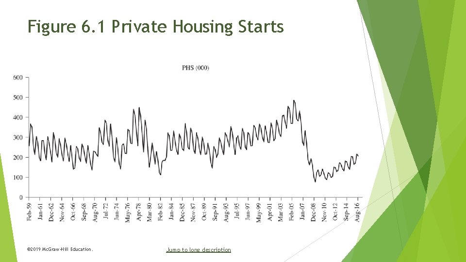
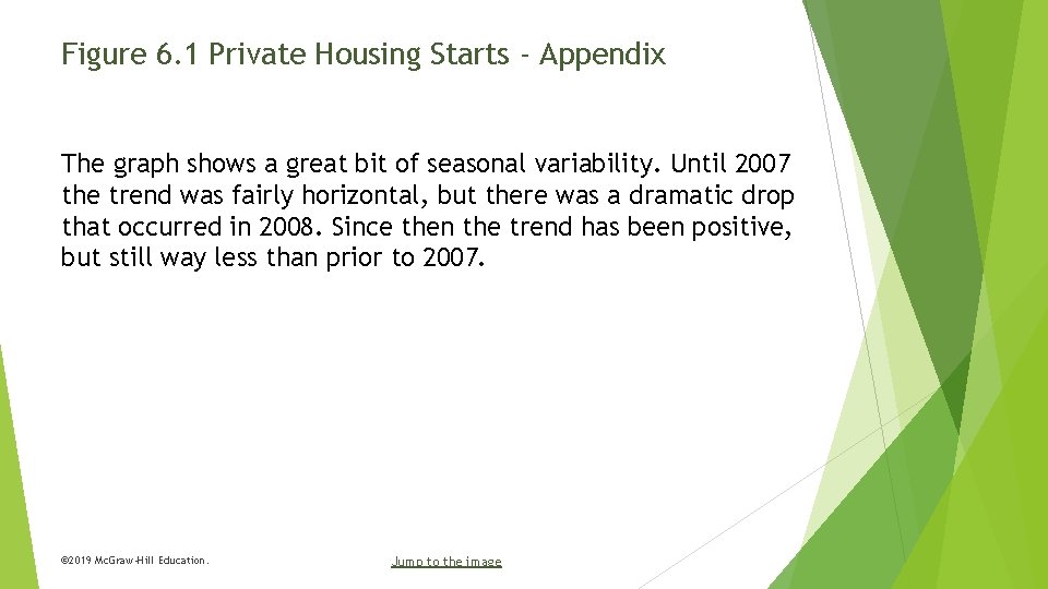
Figure 6. 1 Private Housing Starts © 2019 Mc. Graw-Hill Education. Jump to long description

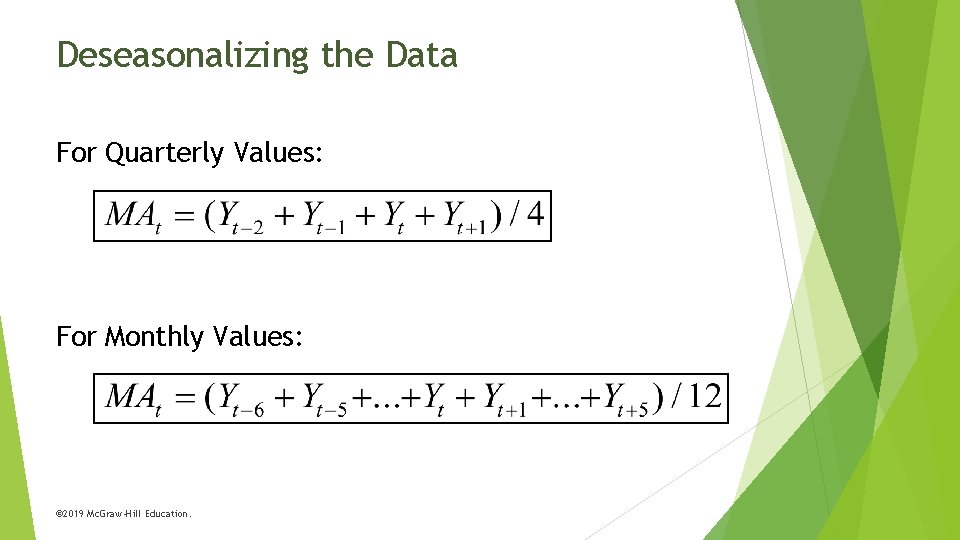
Deseasonalizing the Data For Quarterly Values: For Monthly Values: © 2019 Mc. Graw-Hill Education.

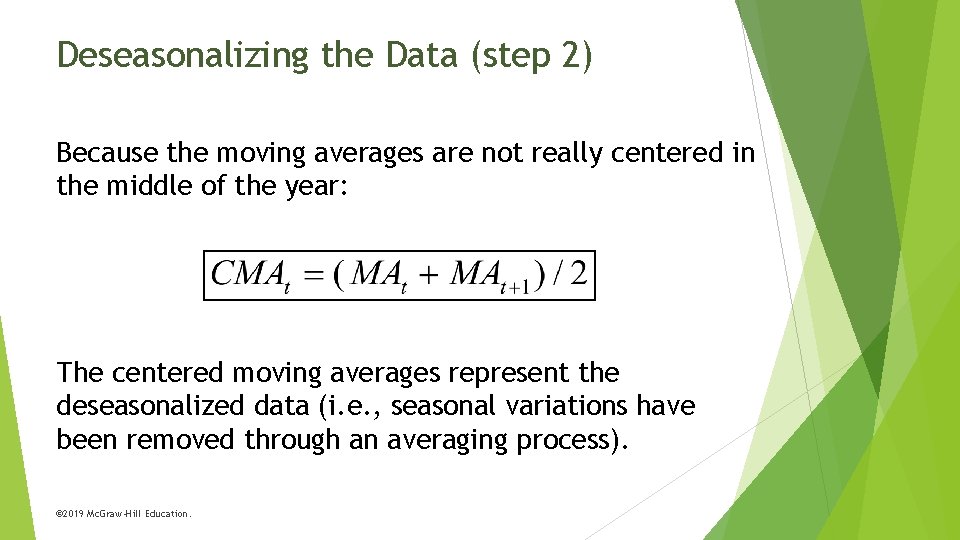
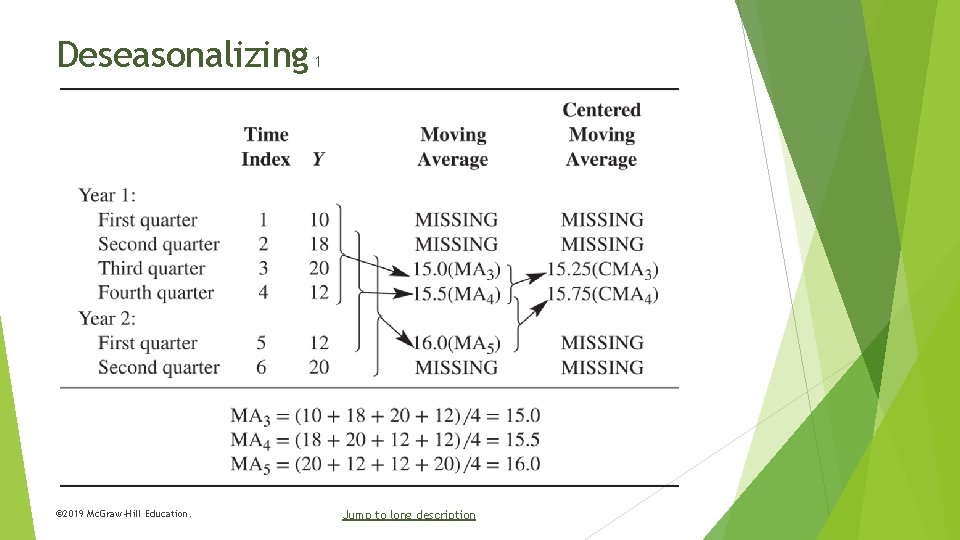
Deseasonalizing the Data (step 2) Because the moving averages are not really centered in the middle of the year: The centered moving averages represent the deseasonalized data (i. e. , seasonal variations have been removed through an averaging process). © 2019 Mc. Graw-Hill Education.

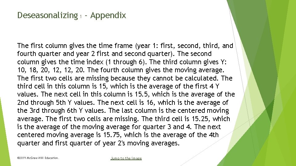
Deseasonalizing 1 © 2019 Mc. Graw-Hill Education. Jump to long description

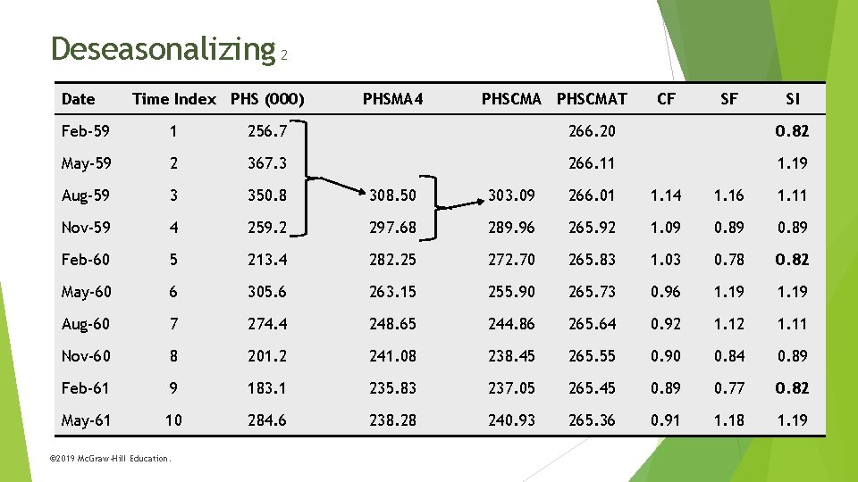
Deseasonalizing 2 Date Time Index PHS (000) PHSMA 4 PHSCMAT CF SF SI Feb-59 1 256. 7 266. 20 0. 82 May-59 2 367. 3 266. 11 1. 19 Aug-59 3 350. 8 308. 50 303. 09 266. 01 1. 14 1. 16 1. 11 Nov-59 4 259. 2 297. 68 289. 96 265. 92 1. 09 0. 89 Feb-60 5 213. 4 282. 25 272. 70 265. 83 1. 03 0. 78 0. 82 May-60 6 305. 6 263. 15 255. 90 265. 73 0. 96 1. 19 Aug-60 7 274. 4 248. 65 244. 86 265. 64 0. 92 1. 11 Nov-60 8 201. 2 241. 08 238. 45 265. 55 0. 90 0. 84 0. 89 Feb-61 9 183. 1 235. 83 237. 05 265. 45 0. 89 0. 77 0. 82 May-61 10 284. 6 238. 28 240. 93 265. 36 0. 91 1. 18 1. 19 © 2019 Mc. Graw-Hill Education.

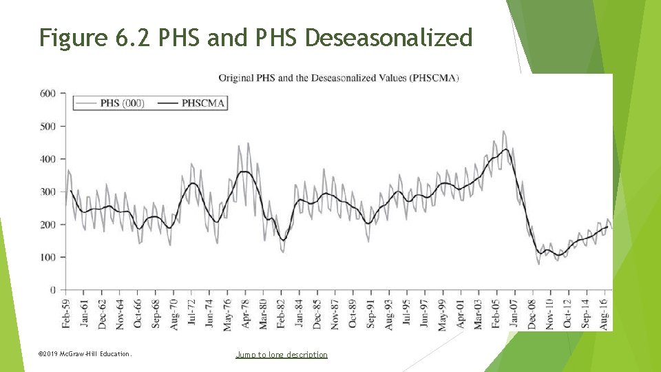
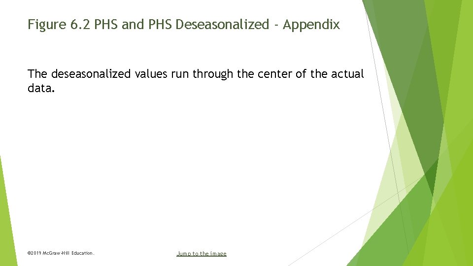
Figure 6. 2 PHS and PHS Deseasonalized © 2019 Mc. Graw-Hill Education. Jump to long description

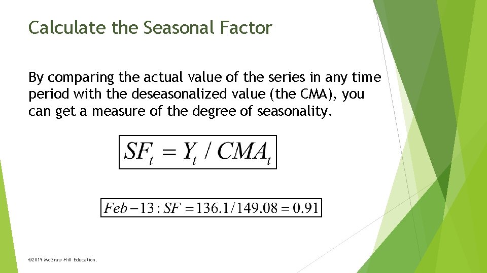
Calculate the Seasonal Factor By comparing the actual value of the series in any time period with the deseasonalized value (the CMA), you can get a measure of the degree of seasonality. © 2019 Mc. Graw-Hill Education.

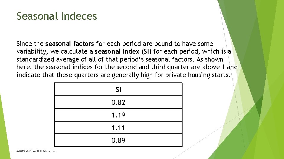
Seasonal Indeces Since the seasonal factors for each period are bound to have some variability, we calculate a seasonal index (SI) for each period, which is a standardized average of all of that period’s seasonal factors. As shown here, the seasonal indices for the second and third quarter are above 1 and indicate that these quarters are generally high for private housing starts. SI 0. 82 1. 19 1. 11 0. 89 © 2019 Mc. Graw-Hill Education.

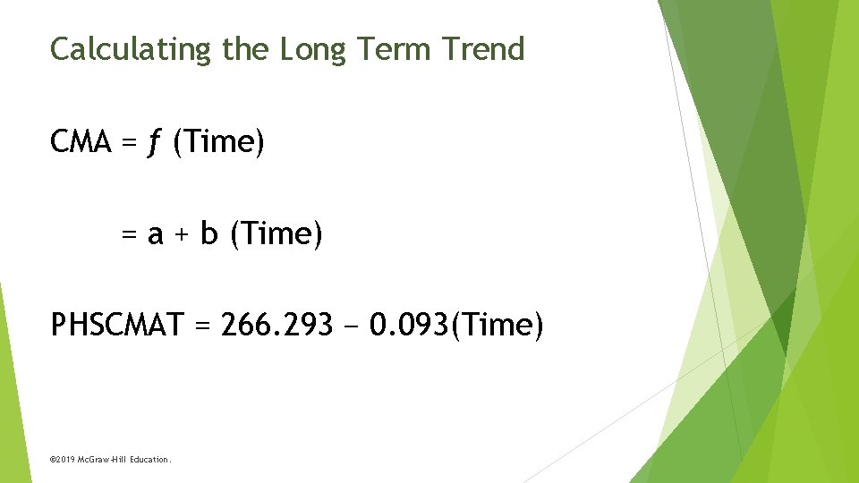
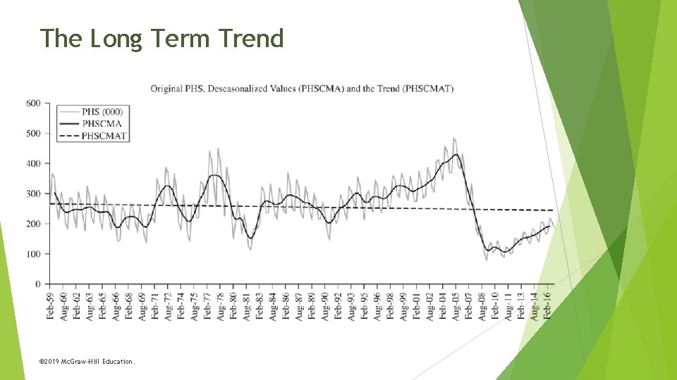
Calculating the Long Term Trend CMA = f (Time) = a + b (Time) PHSCMAT = 266. 293 − 0. 093(Time) © 2019 Mc. Graw-Hill Education.

The Long Term Trend © 2019 Mc. Graw-Hill Education.

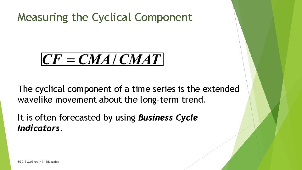
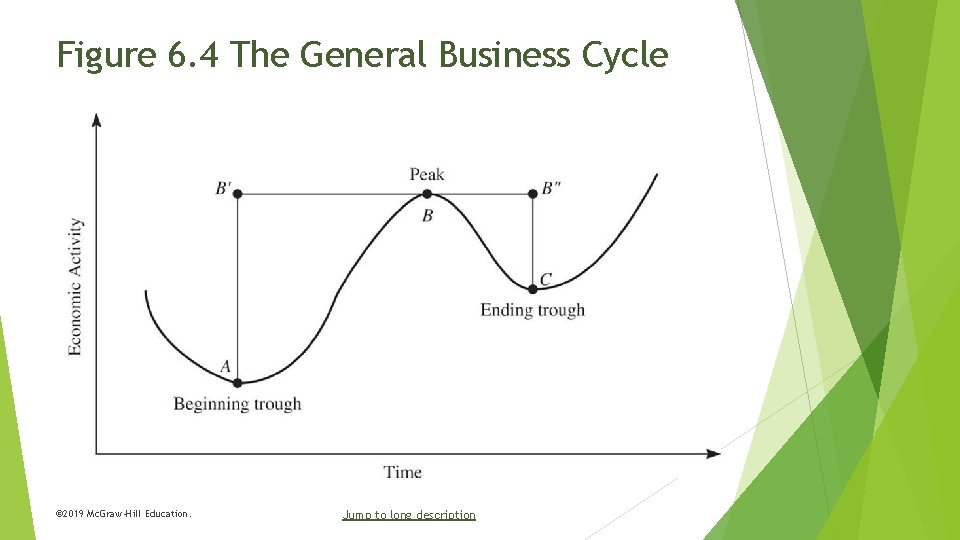
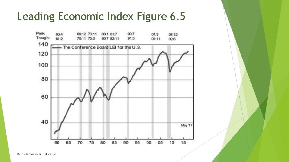
Measuring the Cyclical Component The cyclical component of a time series is the extended wavelike movement about the long-term trend. It is often forecasted by using Business Cycle Indicators. © 2019 Mc. Graw-Hill Education.

Figure 6. 4 The General Business Cycle © 2019 Mc. Graw-Hill Education. Jump to long description

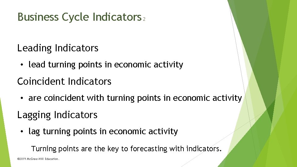
Business Cycle Indicators 1 Developed by NBER Indicators are related to turning points in business cycles Business Cycle defined as "expansions occurring at about the same time in many economic activities" © 2019 Mc. Graw-Hill Education.

Business Cycle Indicators 2 Leading Indicators • lead turning points in economic activity Coincident Indicators • are coincident with turning points in economic activity Lagging Indicators • lag turning points in economic activity Turning points are the key to forecasting with indicators. © 2019 Mc. Graw-Hill Education.

Components of the Composite Leading Index 1 Average weekly hours, manufacturing 2 Average weekly initial claims for unemployment insurance 3 Manufacturers' new orders, consumer goods, and materials 4 ISM® new orders index 5 Manufacturers' new orders, nondefense capital goods excl. aircraft 6 Building permits, new private housing units 7 Stock prices, 500 common stocks 8 Leading Credit Index™ 9 Interest rate spread, 10 -year Treasury bonds less federal funds 10 Avg. consumer expectations for business conditions © 2019 Mc. Graw-Hill Education.

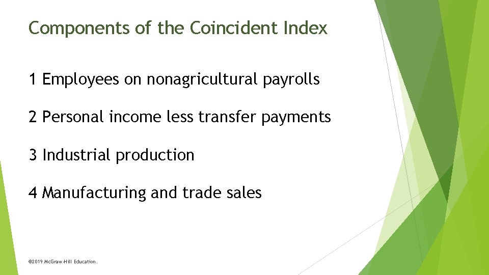
Components of the Coincident Index 1 Employees on nonagricultural payrolls 2 Personal income less transfer payments 3 Industrial production 4 Manufacturing and trade sales © 2019 Mc. Graw-Hill Education.

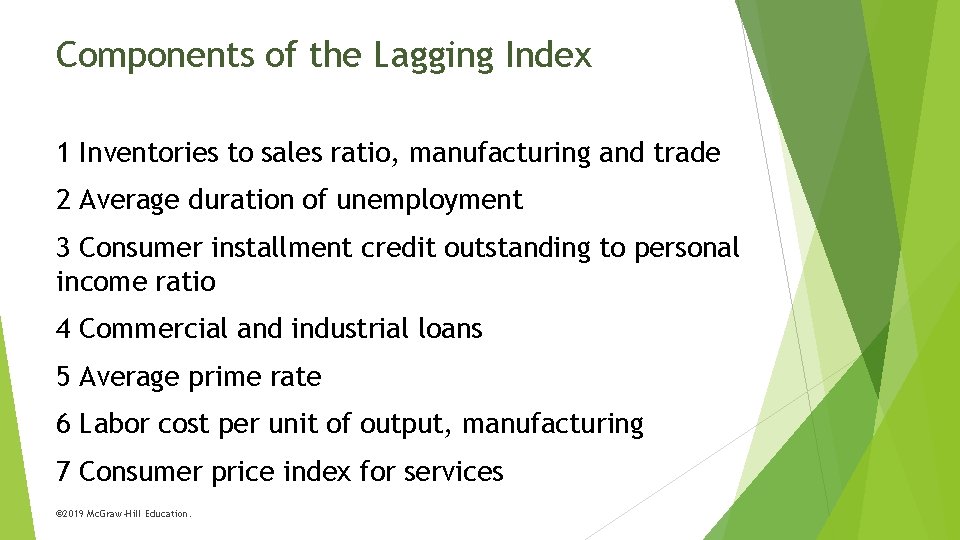
Components of the Lagging Index 1 Inventories to sales ratio, manufacturing and trade 2 Average duration of unemployment 3 Consumer installment credit outstanding to personal income ratio 4 Commercial and industrial loans 5 Average prime rate 6 Labor cost per unit of output, manufacturing 7 Consumer price index for services © 2019 Mc. Graw-Hill Education.

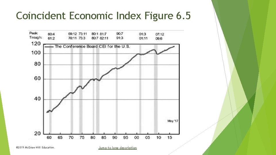
Coincident Economic Index Figure 6. 5 © 2019 Mc. Graw-Hill Education. Jump to long description

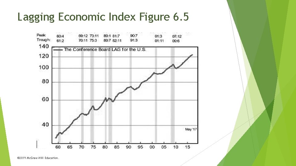
Lagging Economic Index Figure 6. 5 © 2019 Mc. Graw-Hill Education.

Leading Economic Index Figure 6. 5 © 2019 Mc. Graw-Hill Education.

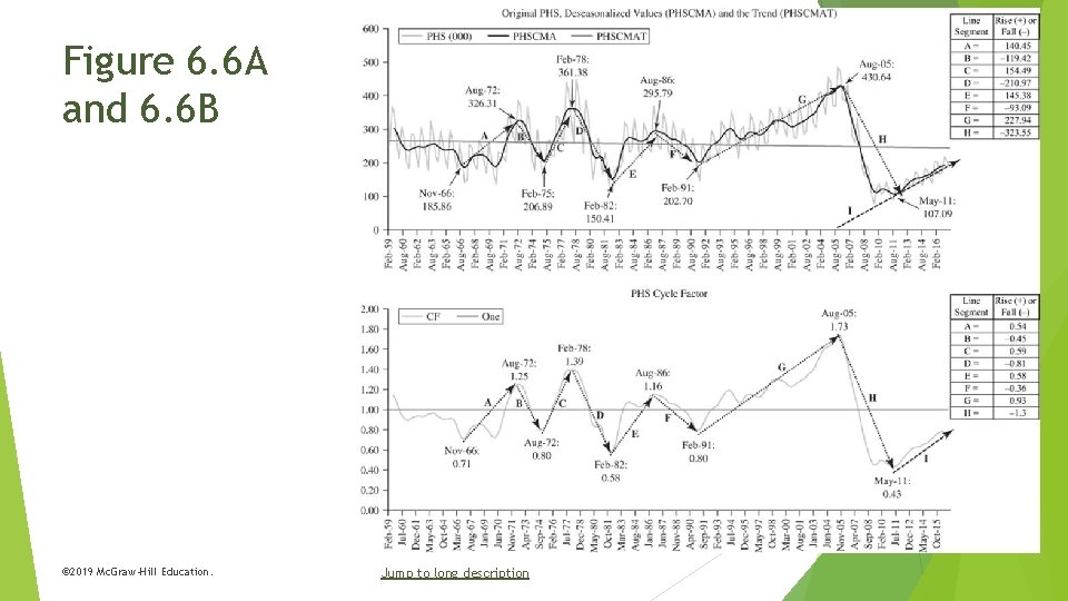
Figure 6. 6 A and 6. 6 B © 2019 Mc. Graw-Hill Education. Jump to long description

The Components Estimated T = The long-term trend based on the deseasonalized data. It is often called the centered moving-average trend (CMAT), since the deseasonalized data are centered moving averages (CMA) of the original Y values. S = Seasonal indices (SI). These are normalized averages of seasonal factors that are determined as the ratio of each period’s actual value (Y) to the deseasonalized value (CMA) for that period. C = The cycle component. The cycle factor (CF) is the ratio of CMA to CMAT and represents the gradual wavelike movements in the series around the trend line. I = The irregular component. This is assumed equal to 1 unless the forecaster has reason to believe a shock may take place, in which case I could be different from 1 for all or part of the forecast period. © 2019 Mc. Graw-Hill Education.

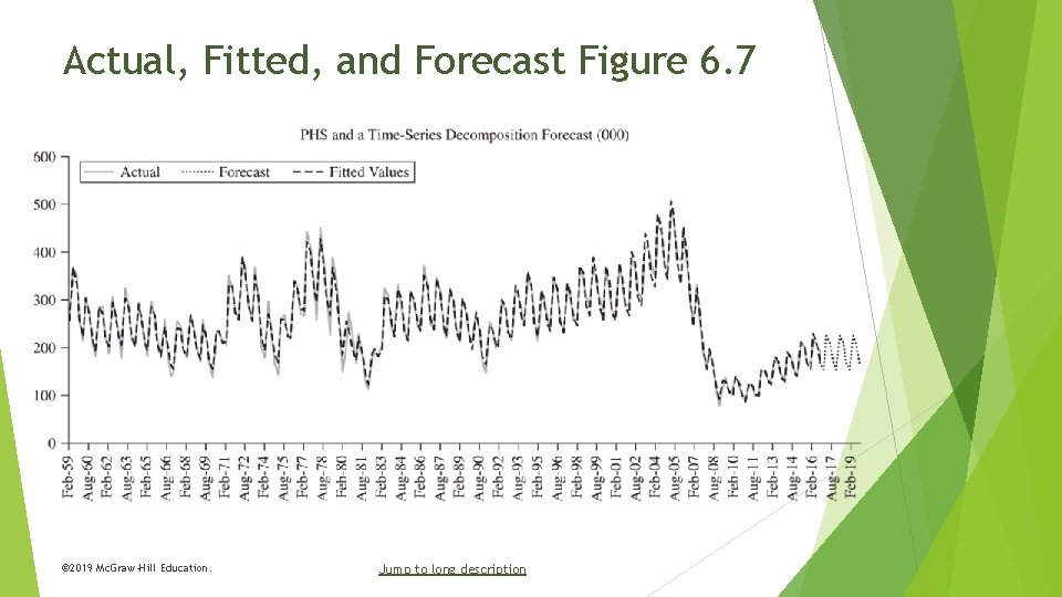
Actual, Fitted, and Forecast Figure 6. 7 © 2019 Mc. Graw-Hill Education. Jump to long description

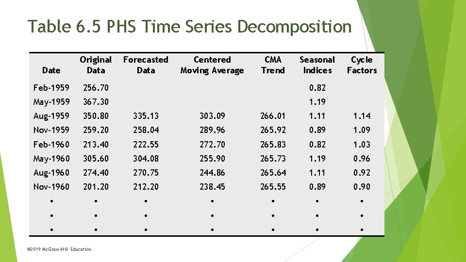
Table 6. 5 PHS Time Series Decomposition Date Original Data Feb-1959 256. 70 0. 82 May-1959 367. 30 1. 19 Aug-1959 350. 80 335. 13 303. 09 266. 01 1. 14 Nov-1959 259. 20 258. 04 289. 96 265. 92 0. 89 1. 09 Feb-1960 213. 40 222. 55 272. 70 265. 83 0. 82 1. 03 May-1960 305. 60 304. 08 255. 90 265. 73 1. 19 0. 96 Aug-1960 274. 40 270. 75 244. 86 265. 64 1. 11 0. 92 Nov-1960 201. 20 212. 20 238. 45 265. 55 0. 89 0. 90 • • • • • • © 2019 Mc. Graw-Hill Education. Forecasted Data Centered Moving Average CMA Trend Seasonal Indices Cycle Factors

Appendix of Image Long Descriptions © 2019 Mc. Graw-Hill Education.

Figure 6. 1 Private Housing Starts - Appendix The graph shows a great bit of seasonal variability. Until 2007 the trend was fairly horizontal, but there was a dramatic drop that occurred in 2008. Since then the trend has been positive, but still way less than prior to 2007. © 2019 Mc. Graw-Hill Education. Jump to the image

Deseasonalizing 1 - Appendix The first column gives the time frame (year 1: first, second, third, and fourth quarter and year 2 first and second quarter). The second column gives the time index (1 through 6). The third column gives Y: 10, 18, 20, 12, 20. The fourth column gives the moving average. The first two cells are missing because they cannot be calculated. The third cell in this column is 15, which is the average of the first 4 Y values. The next cell in this column is 15. 5, which is the average of the 2 nd through 5 th Y values. The next cell is 16, which is the average of the 3 rd through 6 th Y values. The last column is the centered moving average. The first two cells are missing. The third cell is 15. 25, which is the average of the moving average for quarter 3 and 4. The next centered moving average is 15. 75, which is the average of the 4 th quarter and first quarter of year 2's moving averages. © 2019 Mc. Graw-Hill Education. Jump to the image

Figure 6. 2 PHS and PHS Deseasonalized - Appendix The deseasonalized values run through the center of the actual data. © 2019 Mc. Graw-Hill Education. Jump to the image

Figure 6. 4 The General Business Cycle - Appendix This diagram displays time on the horizontal axis and economic activity on the vertical axis. The two minimum points are plotted and are labeled the beginning trough and the ending trough. The peak is between these troughs and lies labeled "B". The troughs are labeled A and C. © 2019 Mc. Graw-Hill Education. Jump to the image

Coincident Economic Index Figure 6. 5 - Appendix Periods of recession are shown with gray vertical bars. The date of each peak and trough for each recession period is provided above each graph. The top graph is the conference board C E I for the U. S. The second graph is the conference board L A G for the U. S. and the bottom graph is the conference board L E I for the U. S. All three graphs show fairly consistent positive trends. © 2019 Mc. Graw-Hill Education. Jump to the image

Figure 6. 6 A and 6. 6 B - Appendix Two time plots showing the private housing starts and deseasonalized value and trends as well as a plot showing just the cycle factors with the deseasonalized values. Line segments are provided throughout the time plot showing the general time periods where the private housing starts rose and fell. The line segments are labeled A through H. The line segments in the first graph rise and fall by the following amounts: A = 140. 45, B = − 119. 42, C = 154. 49, D = − 210. 97, E = 145. 38, F = − 93. 09, G = 227. 94, H = − 323. 55 The line segments in the second graph rise and fall by the following amounts: A = 0. 54, B = − 0. 45, C = 0. 59, D = − 0. 81, E = 0. 58, F = − 0. 36, G = 0. 93, H = − 1. 3 © 2019 Mc. Graw-Hill Education. Jump to the image

Actual, Fitted, and Forecast Figure 6. 7 - Appendix The forecast continues the variation and is fairly horizontal. © 2019 Mc. Graw-Hill Education. Jump to the image