Chapter 6 Efficient Diversification Two Sources of Risk

Chapter 6 Efficient Diversification

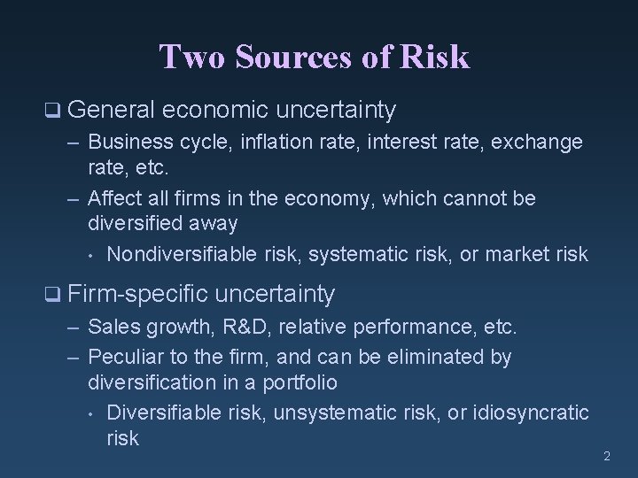
Two Sources of Risk q General economic uncertainty – Business cycle, inflation rate, interest rate, exchange rate, etc. – Affect all firms in the economy, which cannot be diversified away • Nondiversifiable risk, systematic risk, or market risk q Firm-specific uncertainty – Sales growth, R&D, relative performance, etc. – Peculiar to the firm, and can be eliminated by diversification in a portfolio • Diversifiable risk, unsystematic risk, or idiosyncratic risk 2

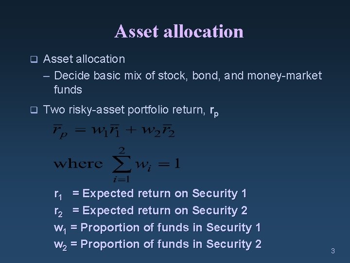
Asset allocation q Asset allocation – Decide basic mix of stock, bond, and money-market funds q Two risky-asset portfolio return, rp r 1 = Expected return on Security 1 r 2 = Expected return on Security 2 w 1 = Proportion of funds in Security 1 w 2 = Proportion of funds in Security 2 3

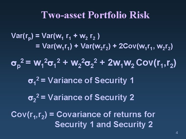
Two-asset Portfolio Risk Var(rp) = Var(w 1 r 1 + w 2 r 2 ) = Var(w 1 r 1) + Var(w 2 r 2) + 2 Cov(w 1 r 1, w 2 r 2) p 2 = w 12 12 + w 22 22 + 2 w 1 w 2 Cov(r 1, r 2) 12 = Variance of Security 1 22 = Variance of Security 2 Cov(r 1, r 2) = Covariance of returns for Security 1 and Security 2 4

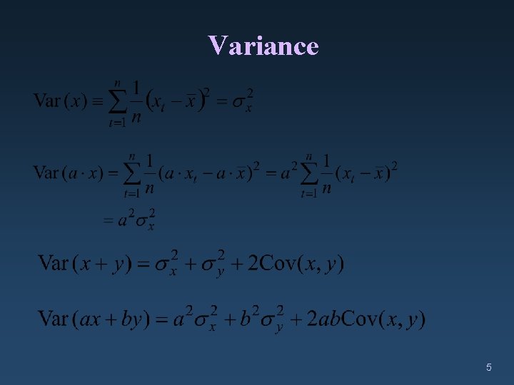
Variance 5

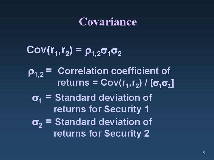
Covariance Cov(r 1, r 2) = 1, 2 = Correlation coefficient of returns = Cov(r 1, r 2) / [ 1 2] 1 = Standard deviation of returns for Security 1 2 = Standard deviation of returns for Security 2 6

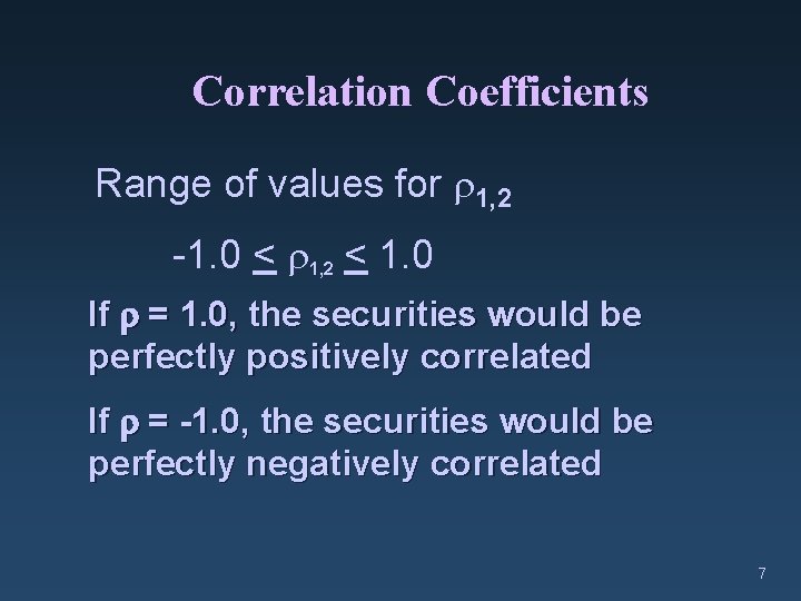
Correlation Coefficients Range of values for 1, 2 -1. 0 < 1, 2 < 1. 0 If = 1. 0, the securities would be perfectly positively correlated If = -1. 0, the securities would be perfectly negatively correlated 7

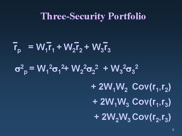
Three-Security Portfolio r p = W 1 r 1 + W 2 r 2 + W 3 r 3 2 p = W 12 12+ W 22 22 + W 32 32 + 2 W 1 W 2 Cov(r 1, r 2) + 2 W 1 W 3 Cov(r 1, r 3) + 2 W 2 W 3 Cov(r 2, r 3) 8

In General, n-Security Portfolio rp = Weighted average of the n-securities’ returns p 2 = Own variance terms + all pair-wise covariances 9

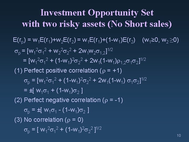
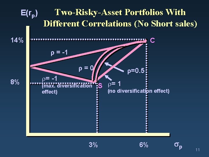
Investment Opportunity Set with two risky assets (No Short sales) E(rp) = w 1 E(r 1)+w 2 E(r 2) = w 1 E(r 1)+(1 -w 1)E(r 2) (w 1≥ 0, w 2 ≥ 0) p = [w 12 12 + w 22 22 + 2 w 1 w 2 1, 2]1/2 = [w 12 12 + (1 -w 1)2 22 + 2 w 1(1 -w 1) 1, 2 1 2]1/2 (1) Perfect positive correlation ( = +1) p = [w 12 12 + (1 -w 1)2 22 + 2 w 1(1 -w 1) 1 2]1/2 = ±[ w 1 1 + (1 -w 1) 2 ] (2) Perfect negative correlation ( = -1) p = ±[ w 1 1 - (1 -w 1) 2 ] (3) No correlation ( = 0) p = [ w 12 12 + (1 -w 1)2 22 ]1/2 10

E(rp) Two-Risky-Asset Portfolios With Different Correlations (No Short sales) 14% C = -1 =0 8% = -1 (max. diversification effect) =0. 5 S = 1 3% (no diversification effect) 6% p 11

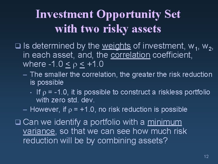
Investment Opportunity Set with two risky assets q Is determined by the weights of investment, w 1, w 2, in each asset, and, the correlation coefficient, where -1. 0 < < +1. 0 – The smaller the correlation, the greater the risk reduction is possible • If = -1. 0, it is possible to construct a riskless portfolio with zero std. dev. – However, if = +1. 0, no risk reduction is possible q Can we identify a portfolio with a minimum variance, so that we can see how much risk reduction will be by combining assets? 12

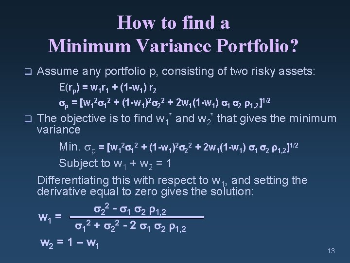
How to find a Minimum Variance Portfolio? q Assume any portfolio p, consisting of two risky assets: E(rp) = w 1 r 1 + (1 -w 1) r 2 p = [w 12 12 + (1 -w 1)2 22 + 2 w 1(1 -w 1) 1 2 1, 2]1/2 q The objective is to find w 1* and w 2* that gives the minimum variance Min. p = [w 12 12 + (1 -w 1)2 22 + 2 w 1(1 -w 1) 1 2 1, 2]1/2 Subject to w 1 + w 2 = 1 Differentiating this with respect to w 1, and setting the derivative equal to zero gives the solution: 22 - 1 2 1, 2 w 1 = 12 + 22 - 2 1, 2 w 2 = 1 – w 1 13

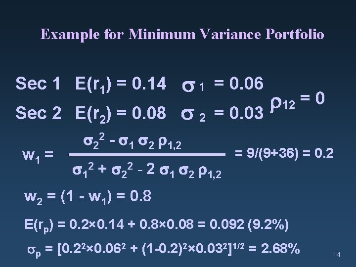
Example for Minimum Variance Portfolio 1 = 0. 06 12 = 0 Sec 2 E(r 2) = 0. 08 2 = 0. 03 Sec 1 E(r 1) = 0. 14 w 1 = 22 - 1 2 1, 2 12 + 22 - 2 1, 2 = 9/(9+36) = 0. 2 w 2 = (1 - w 1) = 0. 8 E(rp) = 0. 2× 0. 14 + 0. 8× 0. 08 = 0. 092 (9. 2%) p = [0. 22× 0. 062 + (1 -0. 2)2× 0. 032]1/2 = 2. 68% 14

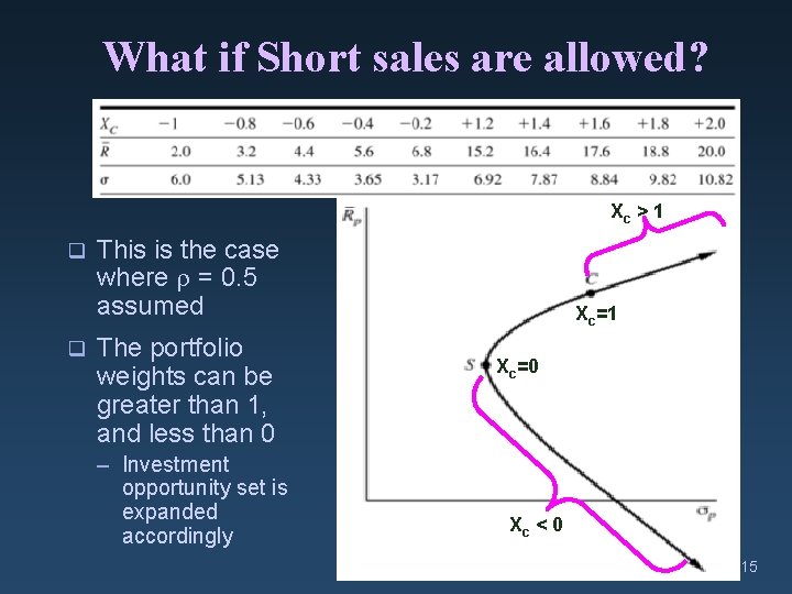
What if Short sales are allowed? Xc > 1 q q This is the case where = 0. 5 assumed The portfolio weights can be greater than 1, and less than 0 – Investment opportunity set is expanded accordingly Xc=1 Xc=0 Xc < 0 15

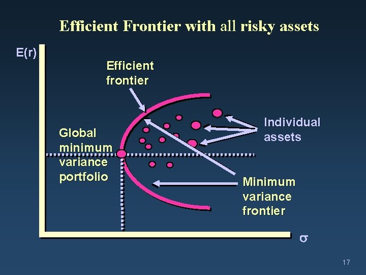
Extending Concepts to All Risky Assets : Markowitz’s Efficient Frontier q For a given level of expected returns, the optimal portfolios are those with the lowest level of risk – This optimal trade-off is described by the portfolios on the efficient frontier, which dominate all other portfolios in the mean-std dev space – This is based on the assumption that investors care only about the means and variances of the returns of their portfolios over a particular period • Investors prefer higher wealth • Investors are risk-averse, and prefer lower risk • The risk can be summarized by the variance (e. g. the return is normally distributed) 16

Efficient Frontier with all risky assets E(r) Efficient frontier Global minimum variance portfolio Individual assets Minimum variance frontier 17

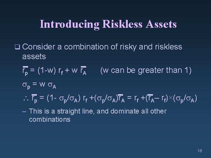
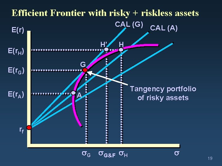
Introducing Riskless Assets q Consider a combination of risky and riskless assets rp = (1 -w) rf + w r. A (w can be greater than 1) p = w A rp = (1 - p/ A) rf +( p/ A)r. A = rf +(r. A– rf)×( p/ A) – This is a straight line, and dominate all other combinations 18

Efficient Frontier with risky + riskless assets CAL (G) CAL (A) E(r) H’ E(r. H) E(r. G) E(r. A) H G A Tangency portfolio of risky assets rf G G&F H 19

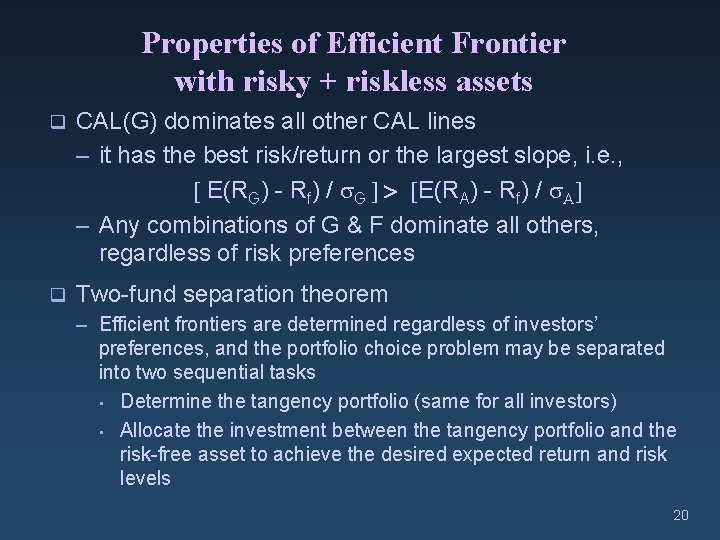
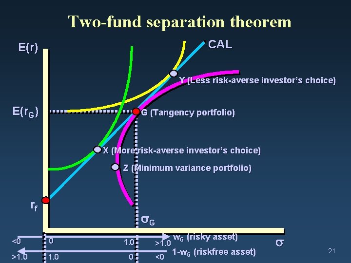
Properties of Efficient Frontier with risky + riskless assets q CAL(G) dominates all other CAL lines – it has the best risk/return or the largest slope, i. e. , [ E(RG) - Rf) / G ] > [E(RA) - Rf) / A] – Any combinations of G & F dominate all others, regardless of risk preferences q Two-fund separation theorem – Efficient frontiers are determined regardless of investors’ preferences, and the portfolio choice problem may be separated into two sequential tasks • Determine the tangency portfolio (same for all investors) • Allocate the investment between the tangency portfolio and the risk-free asset to achieve the desired expected return and risk levels 20

Two-fund separation theorem CAL E(r) Y (Less risk-averse investor’s choice) E(r. G) G (Tangency portfolio) X (More risk-averse investor’s choice) Z (Minimum variance portfolio) rf <0 >1. 0 G 0 1. 0 0 >1. 0 <0 w. G (risky asset) 1 -w. G (riskfree asset) 21

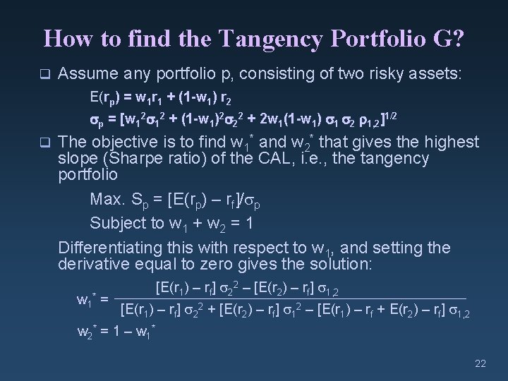
How to find the Tangency Portfolio G? q Assume any portfolio p, consisting of two risky assets: E(rp) = w 1 r 1 + (1 -w 1) r 2 p = [w 12 12 + (1 -w 1)2 22 + 2 w 1(1 -w 1) 1 2 1, 2]1/2 q The objective is to find w 1* and w 2* that gives the highest slope (Sharpe ratio) of the CAL, i. e. , the tangency portfolio Max. Sp = [E(rp) – rf]/ p Subject to w 1 + w 2 = 1 Differentiating this with respect to w 1, and setting the derivative equal to zero gives the solution: w 1 * = [E(r 1) – rf] 22 – [E(r 2) – rf] 1, 2 [E(r 1) – rf] 22 + [E(r 2) – rf] 12 – [E(r 1) – rf + E(r 2) – rf] 1, 2 w 2* = 1 – w 1* 22

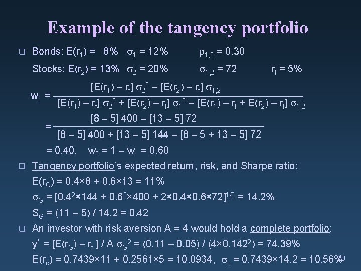
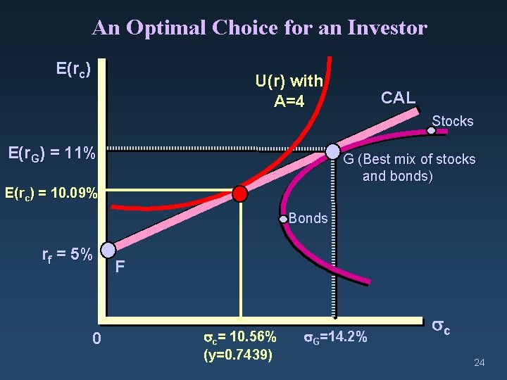
Example of the tangency portfolio q Bonds: E(r 1) = 8% 1 = 12% 1, 2 = 0. 30 Stocks: E(r 2) = 13% 2 = 20% 1, 2 = 72 w 1 = = [E(r 1) – rf] 22 – [E(r 2) – rf] 1, 2 [E(r 1) – rf] 22 + [E(r 2) – rf] 12 – [E(r 1) – rf + E(r 2) – rf] 1, 2 [8 – 5] 400 – [13 – 5] 72 [8 – 5] 400 + [13 – 5] 144 – [8 – 5 + 13 – 5] 72 = 0. 40, q rf = 5% w 2 = 1 – w 1 = 0. 60 Tangency portfolio’s expected return, risk, and Sharpe ratio: E(r. G) = 0. 4× 8 + 0. 6× 13 = 11% G = [0. 42× 144 + 0. 62× 400 + 2× 0. 4× 0. 6× 72]1/2 = 14. 2% SG = (11 – 5) / 14. 2 = 0. 42 q An investor with risk aversion A = 4 would hold a complete portfolio: y* = [E(r. G) – rf ] / A G 2 = (0. 11 – 0. 05) / (4× 0. 1422) = 74. 39% 23 E(rc) = 0. 7439× 11 + 0. 2561× 5 = 10. 0934, c = 0. 7439× 14. 2 = 10. 56%

An Optimal Choice for an Investor E(rc) U(r) with A=4 CAL Stocks E(r. G) = 11% G (Best mix of stocks and bonds) E(rc) = 10. 09% Bonds rf = 5% 0 F c= 10. 56% (y=0. 7439) G=14. 2% c 24

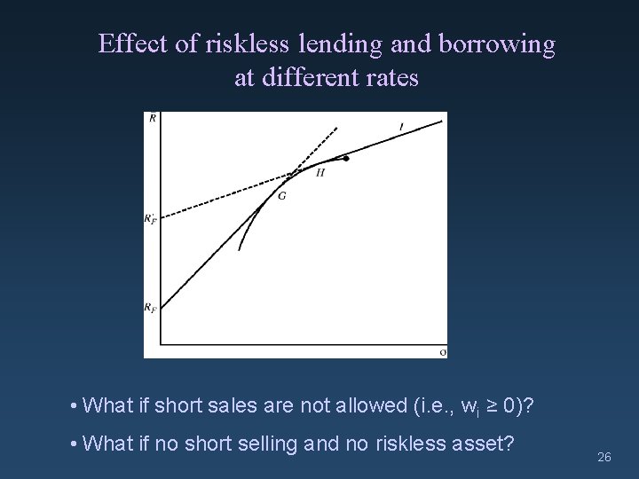
“Asset Allocation Puzzle” q Investors combine the tangent portfolio with cash (riskfree asset) to achieve an efficient frontier, depending on their risk preferences – Conservative investors move more down and to the left along the straight CAL line, and aggressive investors move more up and to the right through borrowing – But, none of the investors can alter the relative proportions of risky assets in the tangency portfolio q In reality, however, most of investment advisors encourage conservative investors to hold disproportionately more bonds relative to stocks, and, vice versa, for aggressive investors. – E. g. cash: bonds: stocks = 50: 30: 20 for conservative investors cash: bonds: stocks = 5: 30: 65 for aggressive investors See Canner, Mankiw, and Weil (1997, AER) q Possible answers: – Aggressive investors cannot borrow at the riskfree rate, and thus, should move along the curved line by allocating more in stocks. – Optimal portfolio for long-term investors would hold more stocks relative to cash (cash is more risky for long-term investors: rollover) 25

Effect of riskless lending and borrowing at different rates • What if short sales are not allowed (i. e. , wi ≥ 0)? • What if no short selling and no riskless asset? 26

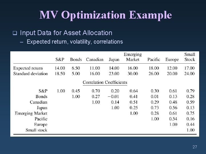
MV Optimization Example q Input Data for Asset Allocation – Expected return, volatility, correlations 27

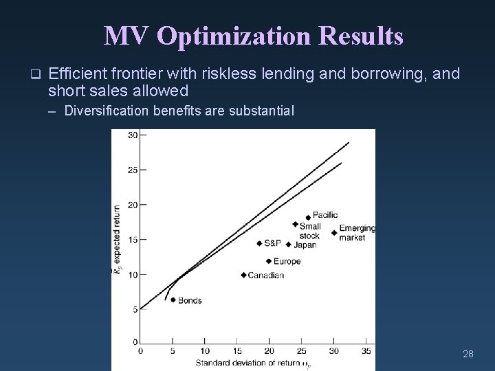
MV Optimization Results q Efficient frontier with riskless lending and borrowing, and short sales allowed – Diversification benefits are substantial 28

Problems with the MV Optimization q Need large amount of input data – Expected return, volatility, correlations q Estimated portfolio weights are sensitive to estimation errors – Small changes in mean returns have large effects on the efficient portfolio weights. (Ex) Jorion (1991, Journal of Banking and Finance) q How long past time-period is necessary for the estimation? – Volatility and correlations change over time q Forecasting variation in volatility and correlations is critical – Investors who can predict changes in volatility better should be able to perform better q Single-period model, without considering rebalancing q Transaction costs such as bid-ask spreads, price pressure (market impact), and brokerage fees should be considered. 29

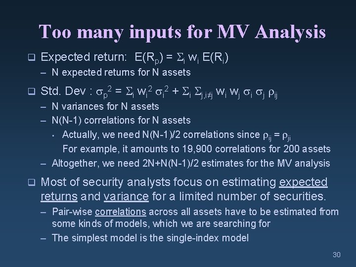
Too many inputs for MV Analysis q Expected return: E(Rp) = i wi E(Ri) – N expected returns for N assets q Std. Dev : p 2 = i wi 2 + i j, i≠j wi wj i j ij – N variances for N assets – N(N-1) correlations for N assets • Actually, we need N(N-1)/2 correlations since ij = ji For example, it amounts to 19, 900 correlations for 200 assets – Altogether, we need 2 N+N(N-1)/2 estimates for the MV analysis q Most of security analysts focus on estimating expected returns and variance for a limited number of securities. – Pair-wise correlations across all assets have to be estimated from some kinds of models, which we are searching for – The simplest model is the single-index model 30

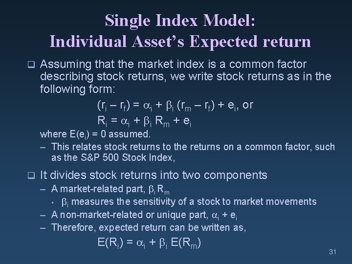
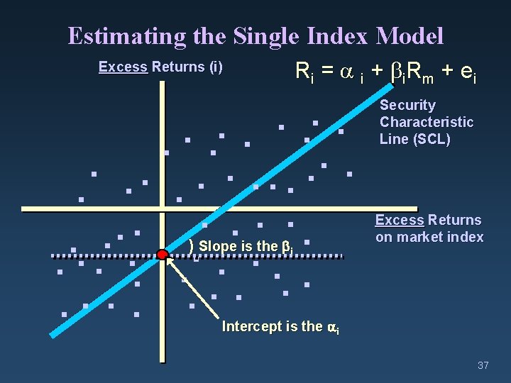
Single Index Model: Individual Asset’s Expected return q Assuming that the market index is a common factor describing stock returns, we write stock returns as in the following form: (ri – rf) = i + i (rm – rf) + ei, or Ri = i + i Rm + ei where E(ei) = 0 assumed. – This relates stock returns to the returns on a common factor, such as the S&P 500 Stock Index, q It divides stock returns into two components – A market-related part, i Rm • i measures the sensitivity of a stock to market movements – A non-market-related or unique part, i + ei – Therefore, expected return can be written as, E(Ri) = i + i E(Rm) 31

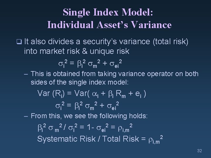
Single Index Model: Individual Asset’s Variance q It also divides a security’s variance (total risk) into market risk & unique risk i 2 = i 2 m 2 + ei 2 – This is obtained from taking variance operator on both sides of the single index model: Var (Ri) = Var( i + i Rm + ei ) i 2 = i 2 m 2 + ei 2 – From this, we see the following holds: i 2 m 2 / i 2 = 1 - ei 2 = i, m 2 Systematic Risk / Total Risk = i, m 2 32

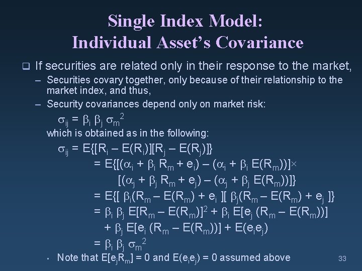
Single Index Model: Individual Asset’s Covariance q If securities are related only in their response to the market, – Securities covary together, only because of their relationship to the market index, and thus, – Security covariances depend only on market risk: ij = i j m 2 which is obtained as in the following: ij = E{[Ri – E(Ri)][Rj – E(Rj)]} = E{[( i + i Rm + ei) – ( i + i E(Rm))]× [( j + j Rm + ej) – ( j + j E(Rm))]} = E{[ i(Rm – E(Rm) + ei ][ j(Rm – E(Rm) + ej ]} = i j E[Rm – E(Rm)]2 + i E[ej (Rm – E(Rm))] + j E[ei (Rm – E(Rm))] + E(eiej) = i j m 2 • Note that E[ej. Rm] = 0 and E(eiej) = 0 assumed above 33

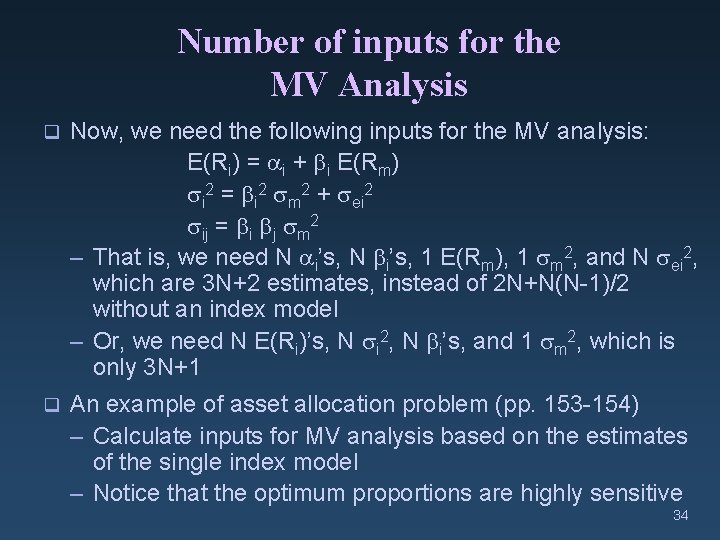
Number of inputs for the MV Analysis q Now, we need the following inputs for the MV analysis: E(Ri) = i + i E(Rm) i 2 = i 2 m 2 + ei 2 ij = i j m 2 – That is, we need N i’s, 1 E(Rm), 1 m 2, and N ei 2, which are 3 N+2 estimates, instead of 2 N+N(N-1)/2 without an index model – Or, we need N E(Ri)’s, N i 2, N i’s, and 1 m 2, which is only 3 N+1 q An example of asset allocation problem (pp. 153 -154) – Calculate inputs for MV analysis based on the estimates of the single index model – Notice that the optimum proportions are highly sensitive 34

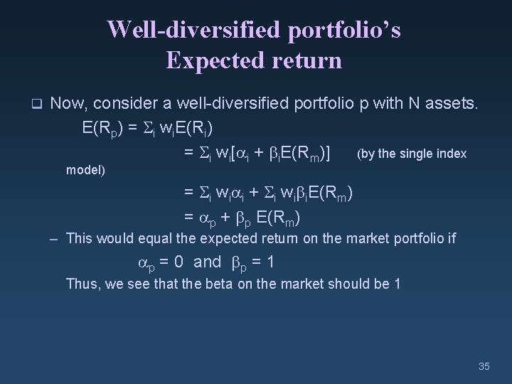
Well-diversified portfolio’s Expected return q Now, consider a well-diversified portfolio p with N assets. E(Rp) = i wi. E(Ri) = i wi[ i + i. E(Rm)] (by the single index model) = i wi i + i wi i. E(Rm) = p + p E(Rm) – This would equal the expected return on the market portfolio if p = 0 and p = 1 Thus, we see that the beta on the market should be 1 35

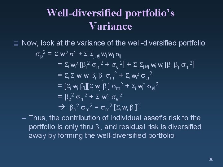
Well-diversified portfolio’s Variance q Now, look at the variance of the well-diversified portfolio: p 2 = i wi 2 + i j, i≠j wi wj ij = i wi 2 [ i 2 m 2 + ei 2] + i j, i≠j wi wj [ i j m 2] = i j wi wj i j m 2 + i wi 2 ei 2 = [ i wi i][ i wj j] m 2 + i wi 2 ei 2 = p 2 m 2 + i wi 2 ei 2 p 2 m 2 = m 2 [ i w i i ] 2 – Thus, the contribution of individual asset’s risk to the portfolio is only thru i, and residual risk is diversified away by forming the well-diversified portfolio 36

Estimating the Single Index Model R i = i + i. R m + e i Excess Returns (i) . . ) Slope is the . . Security Characteristic Line (SCL) Excess Returns on market index i Intercept is the i 37

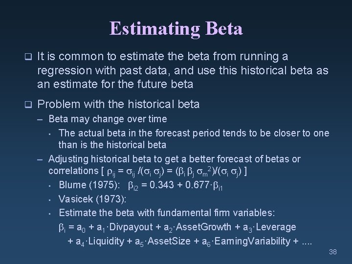
Estimating Beta q It is common to estimate the beta from running a regression with past data, and use this historical beta as an estimate for the future beta q Problem with the historical beta – Beta may change over time • The actual beta in the forecast period tends to be closer to one than is the historical beta – Adjusting historical beta to get a better forecast of betas or correlations [ ij = ij /( i j) = ( i j m 2)/( i j) ] • Blume (1975): i 2 = 0. 343 + 0. 677· i 1 • Vasicek (1973): • Estimate the beta with fundamental firm variables: i = a 0 + a 1·Divpayout + a 2·Asset. Growth + a 3·Leverage + a 4·Liquidity + a 5·Asset. Size + a 6·Earning. Variability +. . 38

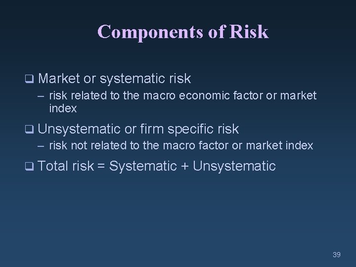
Components of Risk q Market or systematic risk – risk related to the macro economic factor or market index q Unsystematic or firm specific risk – risk not related to the macro factor or market index q Total risk = Systematic + Unsystematic 39

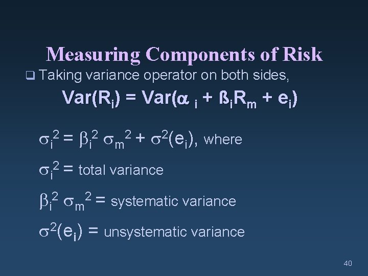
Measuring Components of Risk q Taking variance operator on both sides, Var(Ri) = Var( i + ßi. Rm + ei) i 2 = i 2 m 2 + 2(ei), where i 2 = total variance i 2 m 2 = systematic variance 2(ei) = unsystematic variance 40

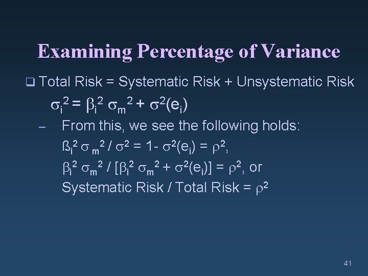
Examining Percentage of Variance q Total Risk = Systematic Risk + Unsystematic Risk i 2 = i 2 m 2 + 2(ei) – From this, we see the following holds: ßi 2 m 2 / 2 = 1 - 2(ei) = 2, i 2 m 2 / [ i 2 m 2 + 2(ei)] = 2, or Systematic Risk / Total Risk = 2 41

In Sum, What are the Advantages of Using the Single Index Model? q Reduces the number of inputs for MV analysis q Increases accuracy of forecasting correlations – (Ex) Elton, Gruber, Urich (1978): Historical correlations were the poorest in forecasting future correlations q Allows security analysts to specialize 42