Chapter 6 Continuous Random Variables Mc GrawHillIrwin Copyright

Chapter 6 Continuous Random Variables Mc. Graw-Hill/Irwin Copyright © 2012 by The Mc. Graw-Hill Companies, Inc. All rights reserved.

Chapter Outline 6. 1 6. 2 Continuous Probability Distributions The Normal Probability Distribution 6 -2

LO 1: Explain what a continuous probability distribution is and how it is used. 6. 1 Continuous Probability Distributions n A continuous random variable may assume any numerical value in one or more intervals n Use a continuous probability distribution to assign probabilities to intervals of values 6 -3

LO 1 Continuous Probability Distributions (Continued) n The curve f(x) is the continuous probability distribution of the continuous random variable x if the probability that x will be in a specified interval is the area under the curve f(x) corresponding to the interval n Other names for a continuous probability distribution: Probability curve n Probability density function n 6 -4

LO 1 Properties of Continuous Probability Distributions n Properties of f(x): f(x) is a continuous function such that 1. 2. f(x) ≥ 0 for all x The total area under the curve of f(x) is equal to 1 n Essential point: An area under a continuous probability distribution is a probability 6 -5

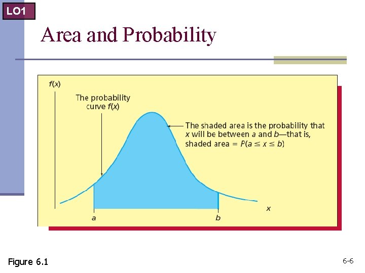
LO 1 Area and Probability Figure 6. 1 6 -6

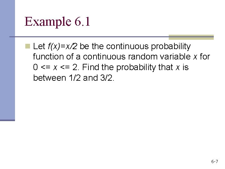
Example 6. 1 n Let f(x)=x/2 be the continuous probability function of a continuous random variable x for 0 <= x <= 2. Find the probability that x is between 1/2 and 3/2. 6 -7

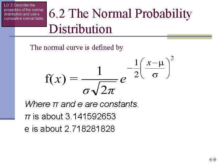
LO 3: Describe the properties of the normal distribution and use a cumulative normal table. 6. 2 The Normal Probability Distribution The normal curve is defined by Where π and e are constants. π is about 3. 141592653 e is about 2. 71828 6 -8

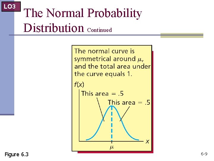
LO 3 The Normal Probability Distribution Continued Figure 6. 3 6 -9

LO 3 Properties of the Normal Distribution 1. The shape of any individual normal curve depends on its specific mean and standard deviation 2. The highest point of f(x) is over the mean. Also the median and mode. 3. The curve is symmetrical about its mean n The left and right halves of the curve are mirror images of each other 6 -10

LO 3 Properties of the Normal Distribution Continued 4. The tails of the normal extend to infinity in both directions n The tails get closer to the horizontal axis but never touch it 5. The area under the normal curve to the right of the mean equals the area under the normal to the left of the mean n The area under each half is 0. 5 6 -11

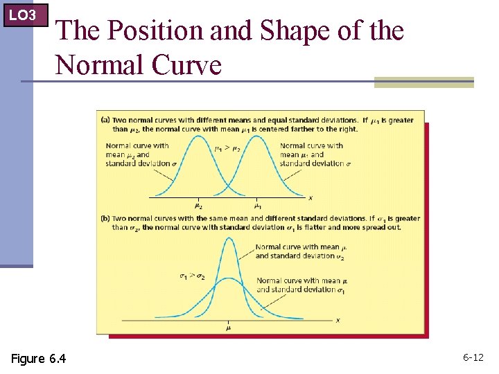
LO 3 The Position and Shape of the Normal Curve Figure 6. 4 6 -12

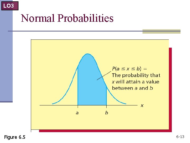
LO 3 Normal Probabilities Figure 6. 5 6 -13

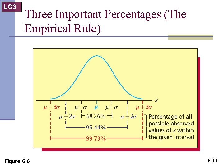
LO 3 Three Important Percentages (The Empirical Rule) Figure 6. 6 6 -14

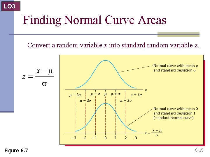
LO 3 Finding Normal Curve Areas Convert a random variable x into standard random variable z. Figure 6. 7 6 -15

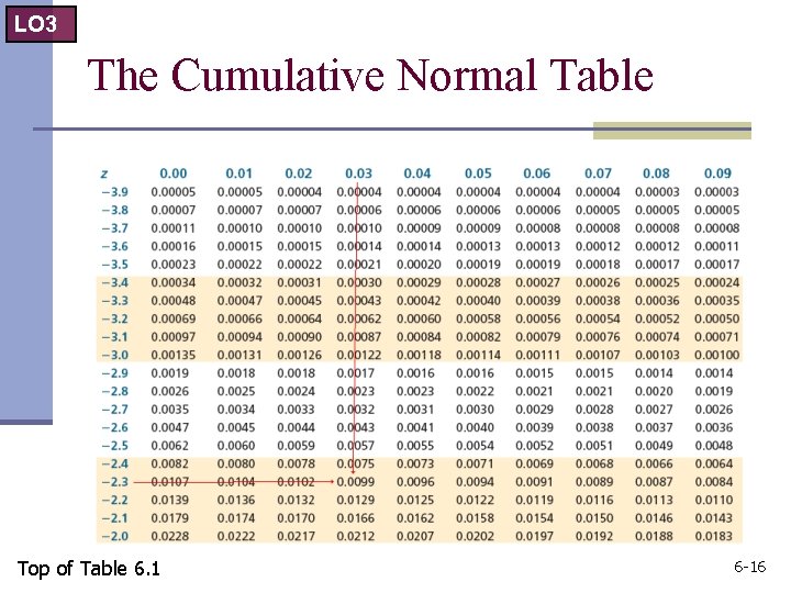
LO 3 The Cumulative Normal Table Top of Table 6. 1 6 -16

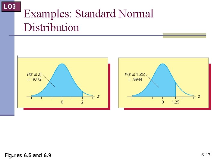
LO 3 Examples: Standard Normal Distribution Figures 6. 8 and 6. 9 6 -17

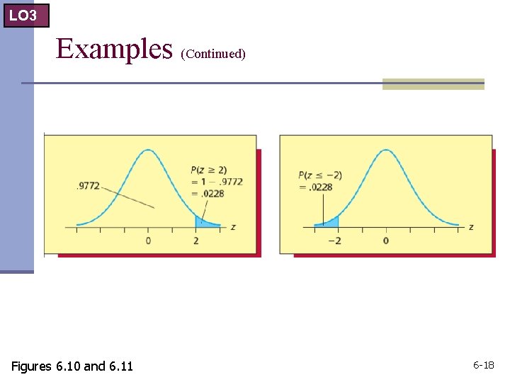
LO 3 Examples (Continued) Figures 6. 10 and 6. 11 6 -18

LO 4: Use the normal distribution to compute probabilities. Finding Normal Probabilities 1. Formulate the problem in terms of x values 2. Calculate the corresponding z values, and restate the problem in terms of these z values 3. Find the required areas under the standard normal curve by using the table Note: It is always useful to draw a picture showing the required areas before using the normal table 6 -19

Example 6. 3 n A plant manager knows that the number of boxes of supplies received weekly is normally distributed with a mean of 200 and a standard deviation of 20. What percentage of the time will the number of boxes received weekly be greater than 210 or less than 180? 6 -20