Chapter 6 Continuous Probability Distributions A visual comparison

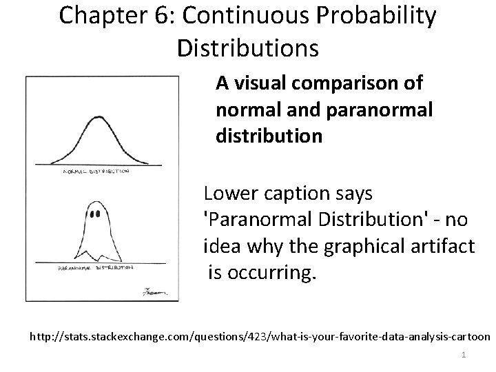
Chapter 6: Continuous Probability Distributions A visual comparison of normal and paranormal distribution Lower caption says 'Paranormal Distribution' - no idea why the graphical artifact is occurring. http: //stats. stackexchange. com/questions/423/what-is-your-favorite-data-analysis-cartoon 1

6. 1: Probability Distributions for a Continuous Random Variable - Goals • Describe the basis of the probability density function (pdf). • Use the probability density function (pdf) and cumulative distribution function (cdf) of a continuous random variable to calculate probabilities and percentiles (median) of events. • Be able to use a pdf to find the mean of a continuous random variable. • Be able to use a pdf to find the variance of a continuous random variable. 2

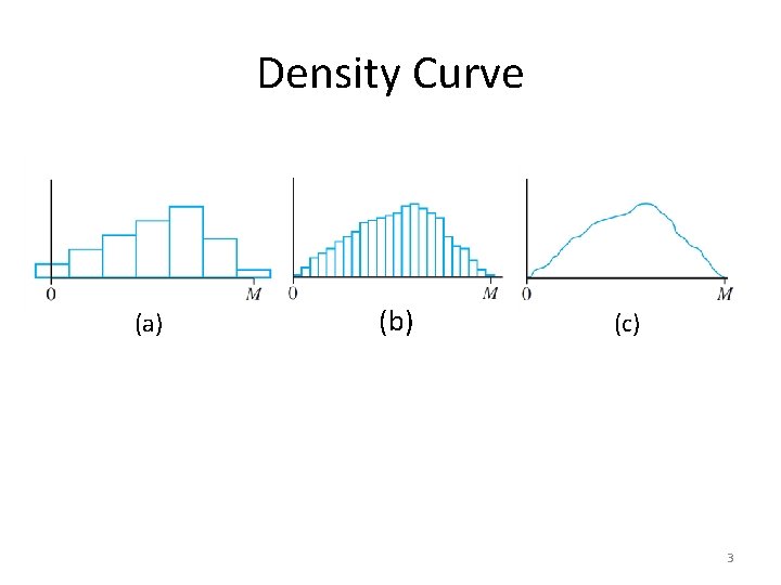
Density Curve (a) (b) (c) 3

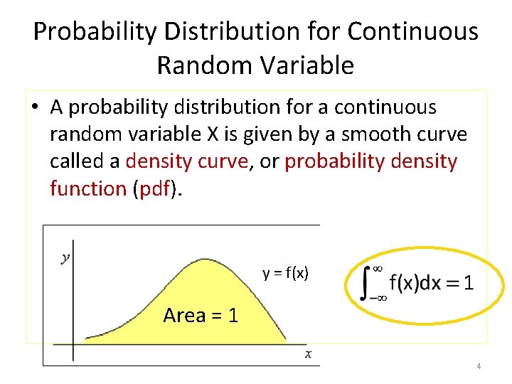
Probability Distribution for Continuous Random Variable • A probability distribution for a continuous random variable X is given by a smooth curve called a density curve, or probability density function (pdf). y = f(x) Area = 1 4

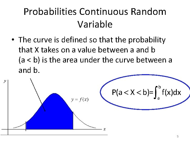
Probabilities Continuous Random Variable • The curve is defined so that the probability that X takes on a value between a and b (a < b) is the area under the curve between a and b. 5

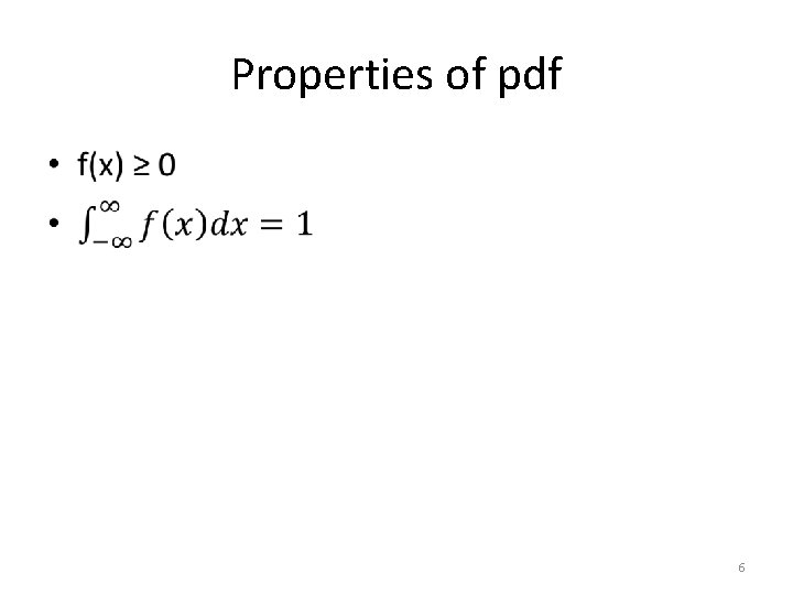
Properties of pdf • 6

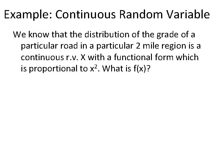
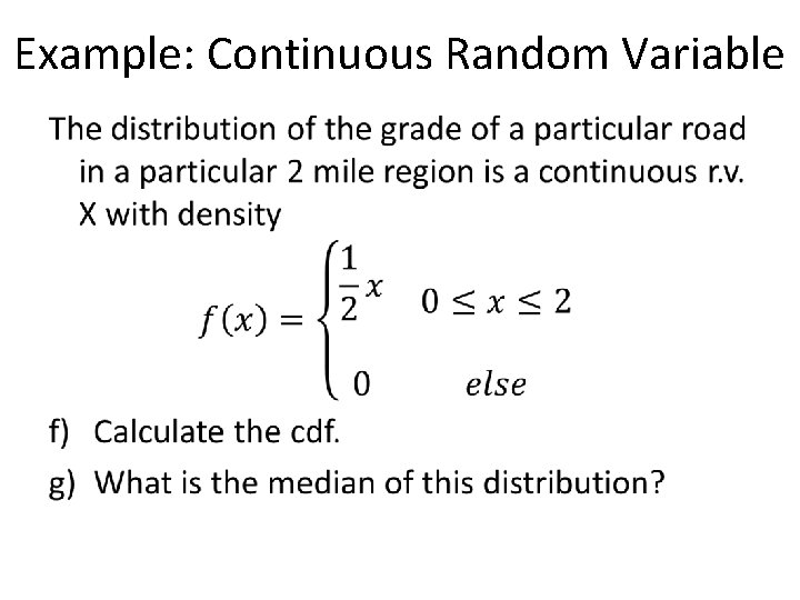
Example: Continuous Random Variable We know that the distribution of the grade of a particular road in a particular 2 mile region is a continuous r. v. X with a functional form which is proportional to x 2. What is f(x)?

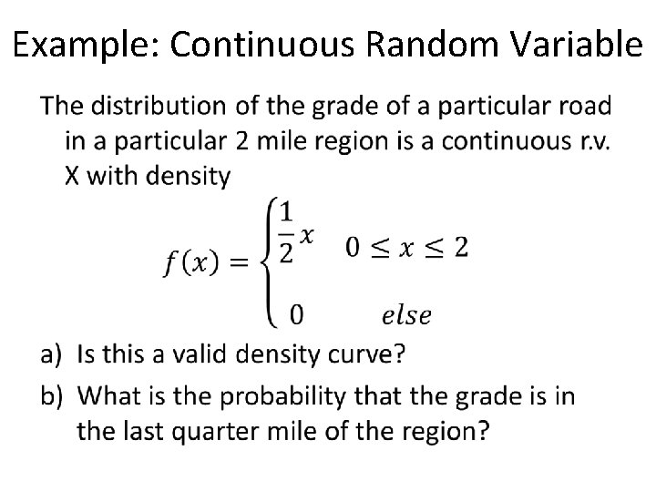
Example: Continuous Random Variable •

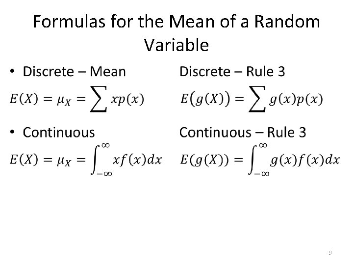
Formulas for the Mean of a Random Variable • 9

Variance of a Random Variable • 10

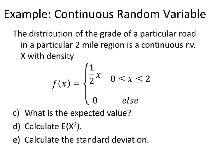
Example: Continuous Random Variable •

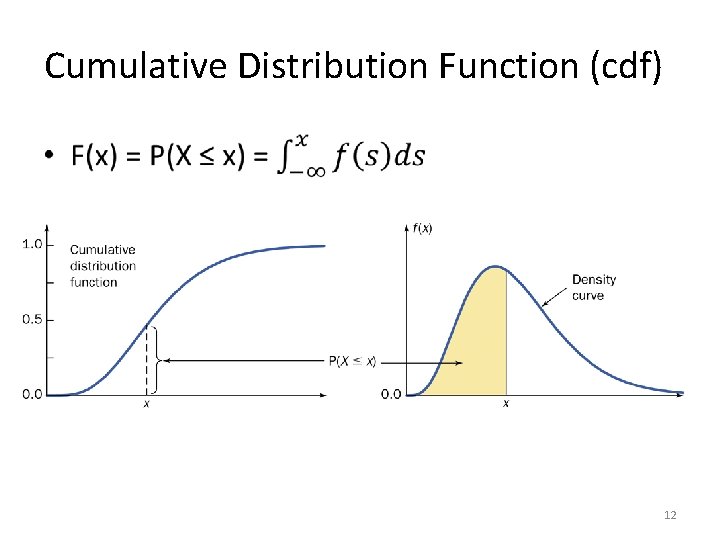
Cumulative Distribution Function (cdf) • 12

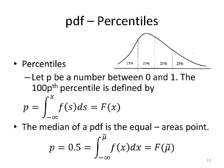
pdf – Percentiles • 13

Example: Continuous Random Variable •

6. 2 Normal Distribution http: //delfe. tumblr. com/ 15

6. 2/6. 5: The Normal Distribution The Normal Approximation to the Binomial Distribution - Goals Be able to sketch the normal distribution. Be able to standardize a value. Be able to use the Z-table. Be able to calculate probabilities. Be able to calculate percentiles (Inverse calculations). • Determine when you can use the normal approximation to the binomial and perform calculations using this approximation. • • • 16

Normal Distribution • 17

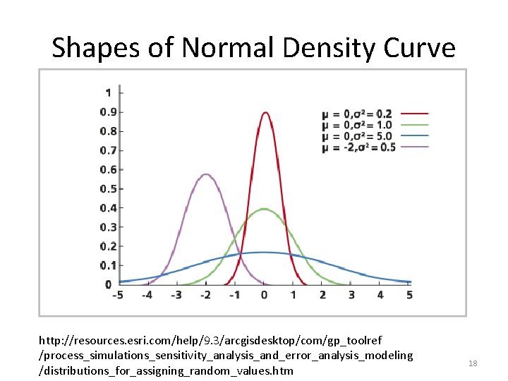
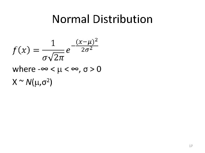
Shapes of Normal Density Curve http: //resources. esri. com/help/9. 3/arcgisdesktop/com/gp_toolref /process_simulations_sensitivity_analysis_and_error_analysis_modeling /distributions_for_assigning_random_values. htm 18

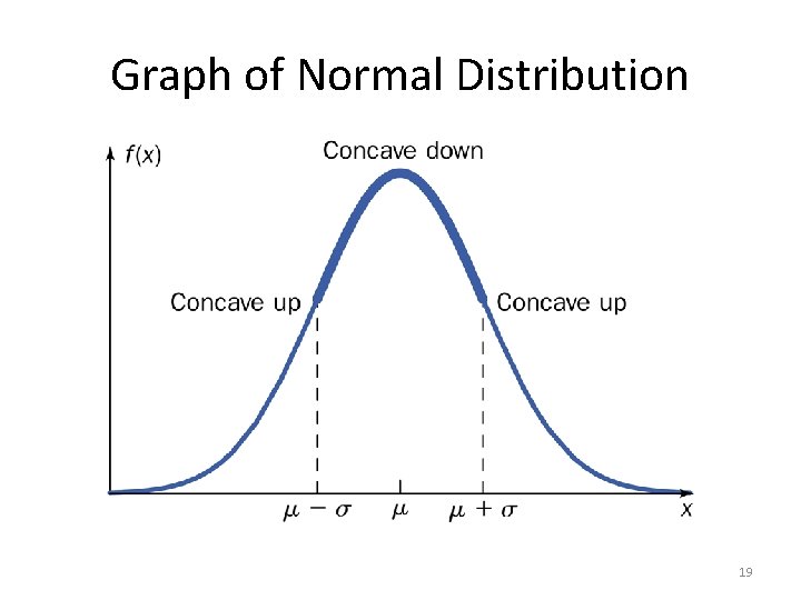
Graph of Normal Distribution 19

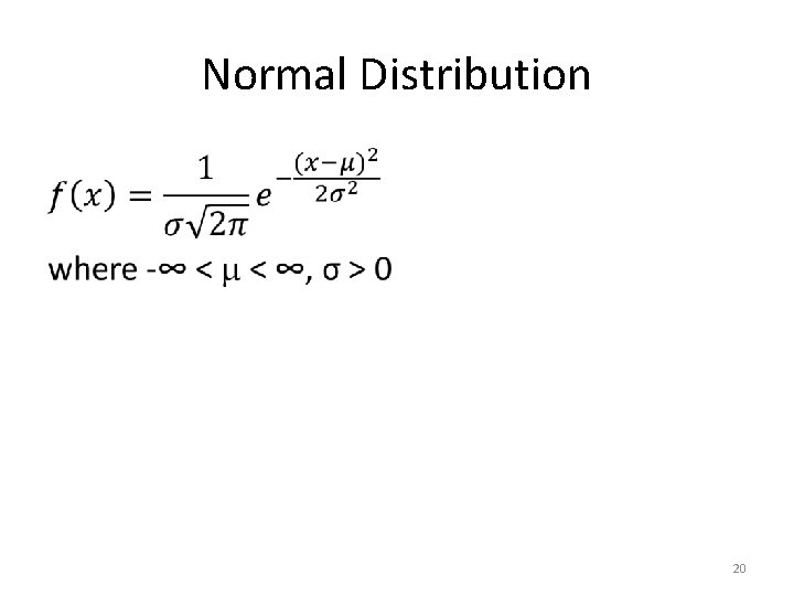
Normal Distribution • 20

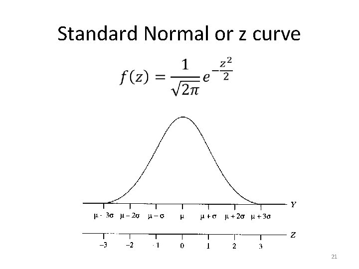
Standard Normal or z curve 21

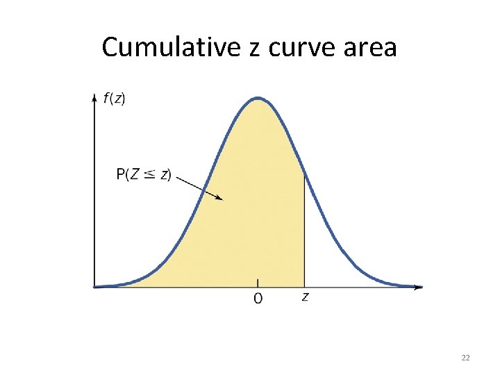
Cumulative z curve area 22

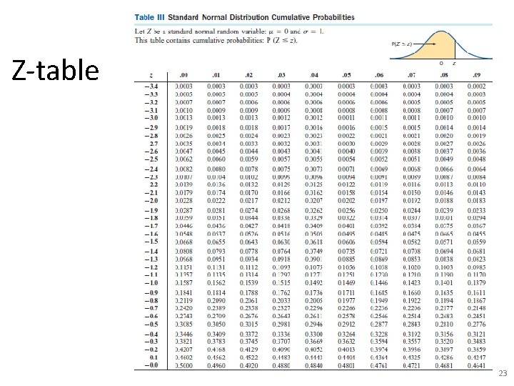
Z-table 23

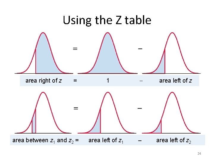
Using the Z table area right of z = area between z 1 and z 2 = 1 area left of z – area left of z 2 24

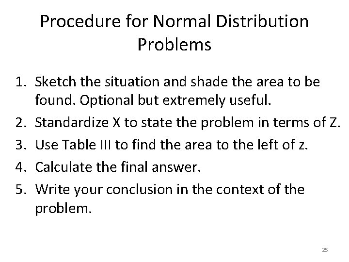
Procedure for Normal Distribution Problems 1. Sketch the situation and shade the area to be found. Optional but extremely useful. 2. Standardize X to state the problem in terms of Z. 3. Use Table III to find the area to the left of z. 4. Calculate the final answer. 5. Write your conclusion in the context of the problem. 25

Normal Distribution: Example A particular rash has shown up in an elementary school. It has been determined that the length of time that the rash will last is normally distributed with mean 6 days and standard deviation 1. 5 days. a) What is the percentage of students that have the rash for longer than 8 days? b) What is the percentage of students that the rash will last between 3. 7 and 8 days? 26

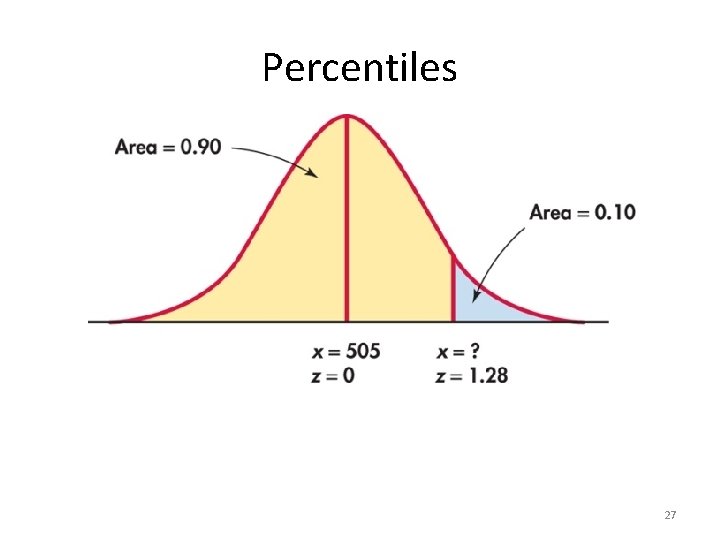
Percentiles 27

Normal Distribution: Example A particular rash has shown up in an elementary school. It has been determined that the length of time that the rash will last is normally distributed with mean 6 days and standard deviation 1. 5 days. c) How long would the student’s rash have to have lasted to be in the top 10% of the number of days that the students have the rash? 28

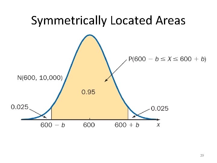
Symmetrically Located Areas 29

Normal Distribution: Example A particular rash has shown up in an elementary school. It has been determined that the length of time that the rash will last is normally distributed with mean 6 days and standard deviation 1. 5 days. d) What interval symmetrically placed about the mean will capture 95% of the times for the student’s rashes to have lasted. 30

Why Approximate the Binomial Distribution? 1. Intervals 2. Computation (n large) 3. Inference 31

Difficulties with the Normal Approximation to the Binomial 1. Skewedness of the Binomial Distribution. 2. The Binomial Distribution is discrete. 32

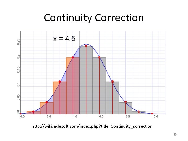
Continuity Correction http: //wiki. axlesoft. com/index. php? title=Continuity_correction 33

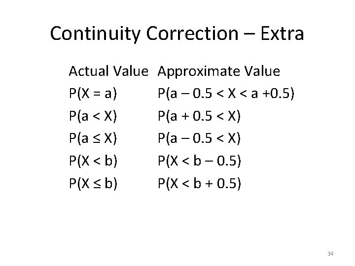
Continuity Correction – Extra Actual Value P(X = a) P(a < X) P(a ≤ X) P(X < b) P(X ≤ b) Approximate Value P(a – 0. 5 < X < a +0. 5) P(a + 0. 5 < X) P(a – 0. 5 < X) P(X < b – 0. 5) P(X < b + 0. 5) 34

Example: Normal Approximation to the Binomial The ideal size of a first-year class at a particular college is 150 students. The college, knowing from past experience that on the average only 30 percent of those accepted for admission will actually attend, uses a policy of approving the applications of 450 students. Compute the probability that more than 150 students attend this college. 35

6. 3: Checking the Normality Assumption- Goals • Be able to state why it is important to be able to check to see whether a data set is normal or not. • Be able to determine if a distribution is normal (normal quantile plots) 36

Methods for Checking Normality 1. 2. 3. 4. Graphs Backward Empirical Rule IQR/s Normal Probability Plot 37

Procedure: Normal Quantile Plot 1) Arrange the data from smallest to largest. 2) Record the corresponding percentiles (quantiles). 3) Find the z value corresponding to the quantile calculated in part 2. 4) Plot the original data points (from 1) vs. the z values (from 3). 38

6. 4: The Exponential Distribution (and Uniform Distribution) - Goals • Be able to recognize situations that may be described by uniform or exponential distributions. • Be able to recognize the sketches of the pdfs for uniform and exponential distribution. • Calculate the probability, mean and standard deviation when X has a uniform or exponential distribution. 39

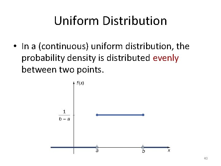
Uniform Distribution • In a (continuous) uniform distribution, the probability density is distributed evenly between two points. 40

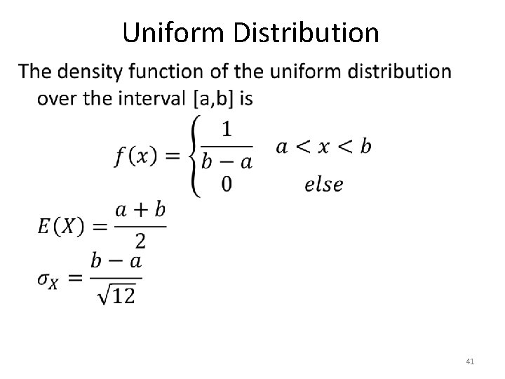
Uniform Distribution • 41

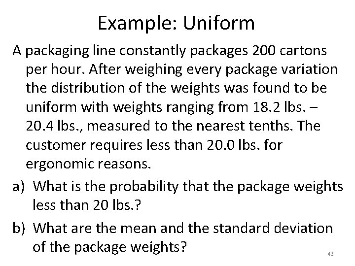
Example: Uniform A packaging line constantly packages 200 cartons per hour. After weighing every package variation the distribution of the weights was found to be uniform with weights ranging from 18. 2 lbs. – 20. 4 lbs. , measured to the nearest tenths. The customer requires less than 20. 0 lbs. for ergonomic reasons. a) What is the probability that the package weights less than 20 lbs. ? b) What are the mean and the standard deviation of the package weights? 42

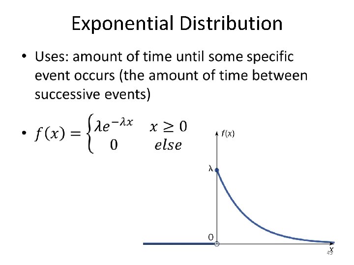
Exponential Distribution • 43

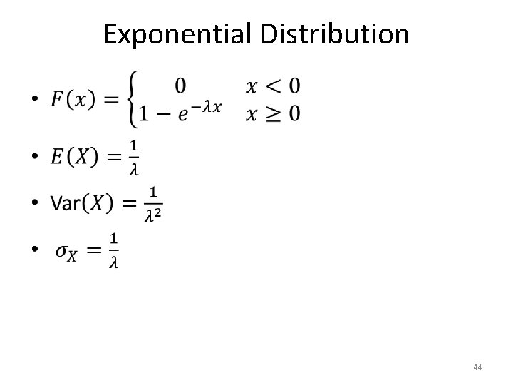
Exponential Distribution • 44

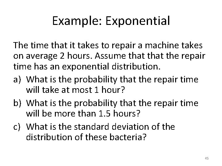
Example: Exponential The time that it takes to repair a machine takes on average 2 hours. Assume that the repair time has an exponential distribution. a) What is the probability that the repair time will take at most 1 hour? b) What is the probability that the repair time will be more than 1. 5 hours? c) What is the standard deviation of the distribution of these bacteria? 45

Gamma Distribution • Generalization of the exponential function • Uses – probability theory – theoretical statistics – actuarial science – operations research – engineering 46

Beta Distribution • This distribution is only defined on an interval – standard beta is on the interval [0, 1] • uses – modeling proportions – percentages – Probabilities • Uniform distribution is a member of this family. 47

Other Continuous Random Variables • Weibull – exponential is a member of family – uses: lifetimes • lognormal – log of the normal distribution – uses: products of distributions • Cauchy – symmetrical, long straggly tails 48