Chapter 6 Continuous Probability Distributions 1 Chapter Outline
Chapter 6 Continuous Probability Distributions 1
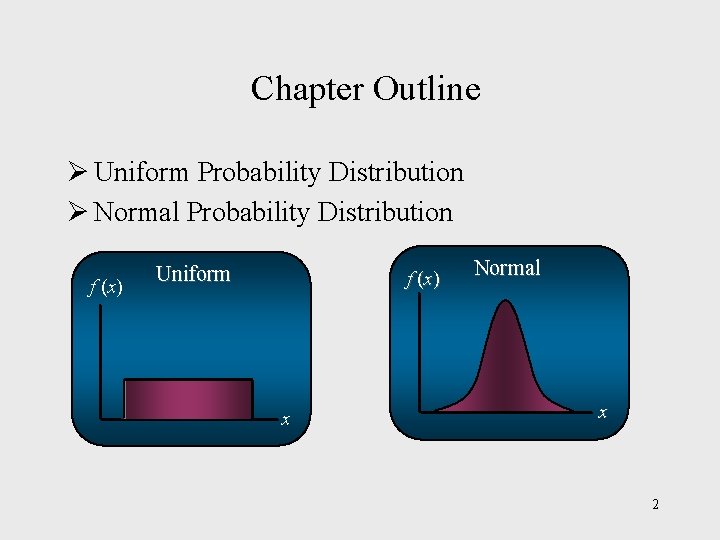
Chapter Outline Ø Uniform Probability Distribution Ø Normal Probability Distribution f (x) Uniform f (x ) x Normal x 2
Continuous Probability Distributions § A continuous random variable assume values that have no gap or jump between them. § Since between any two values, a continuous random variable assumes infinite number of values, the probability that any particular value occurs is zero. § Therefore, we study the probability of the random variable assuming a value within a given interval. 3
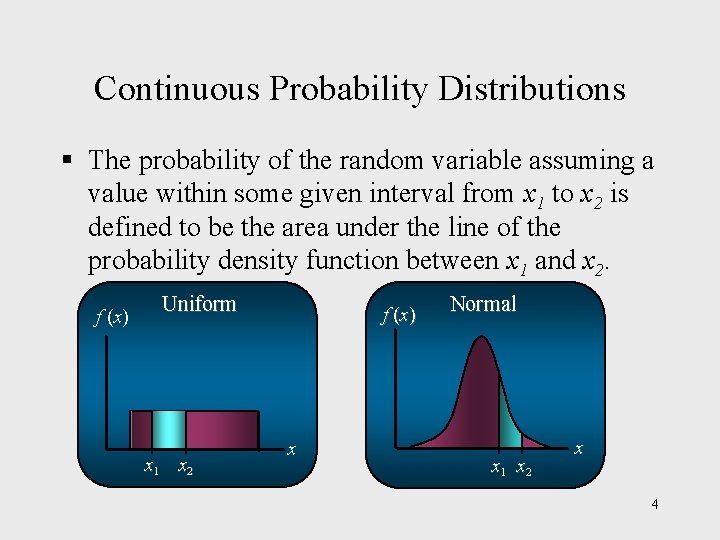
Continuous Probability Distributions § The probability of the random variable assuming a value within some given interval from x 1 to x 2 is defined to be the area under the line of the probability density function between x 1 and x 2. f (x) Uniform x 1 x 2 f (x ) x Normal x 1 x 2 x 4
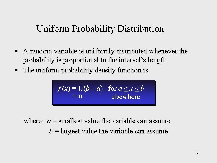
Uniform Probability Distribution § A random variable is uniformly distributed whenever the probability is proportional to the interval’s length. § The uniform probability density function is: f (x) = 1/(b – a) for a < x < b =0 elsewhere: a = smallest value the variable can assume b = largest value the variable can assume 5
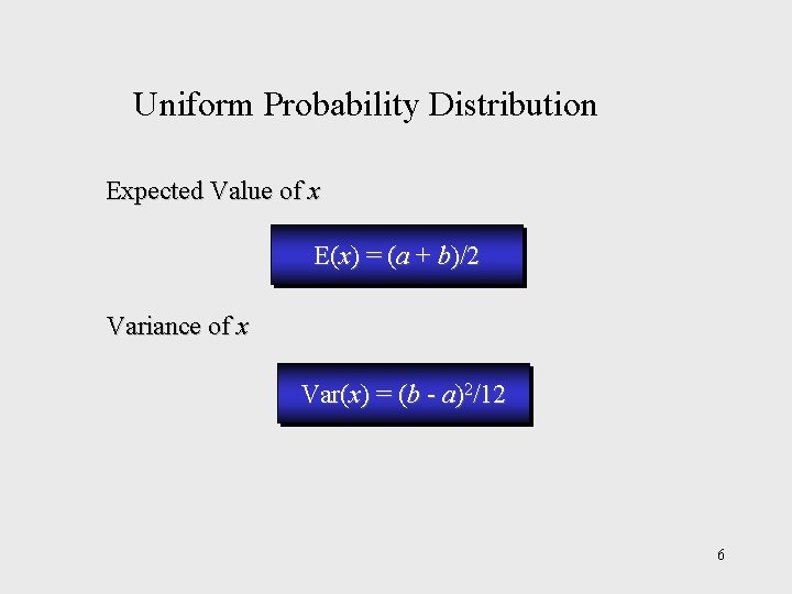
Uniform Probability Distribution Expected Value of x E(x) = (a + b)/2 Variance of x Var(x) = (b - a)2/12 6
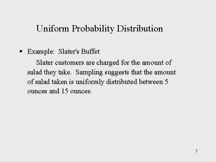
Uniform Probability Distribution § Example: Slater's Buffet Slater customers are charged for the amount of salad they take. Sampling suggests that the amount of salad taken is uniformly distributed between 5 ounces and 15 ounces. 7
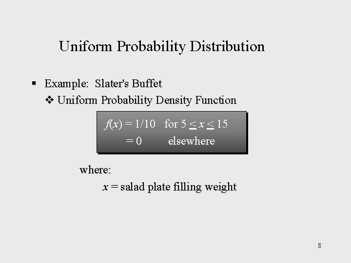
Uniform Probability Distribution § Example: Slater's Buffet v Uniform Probability Density Function f(x) = 1/10 for 5 < x < 15 =0 elsewhere: x = salad plate filling weight 8
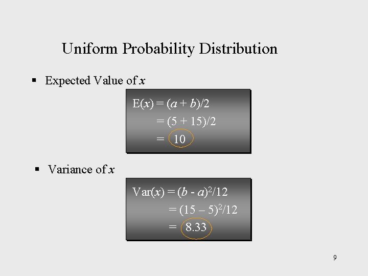
Uniform Probability Distribution § Expected Value of x E(x) = (a + b)/2 = (5 + 15)/2 = 10 § Variance of x Var(x) = (b - a)2/12 = (15 – 5)2/12 = 8. 33 9
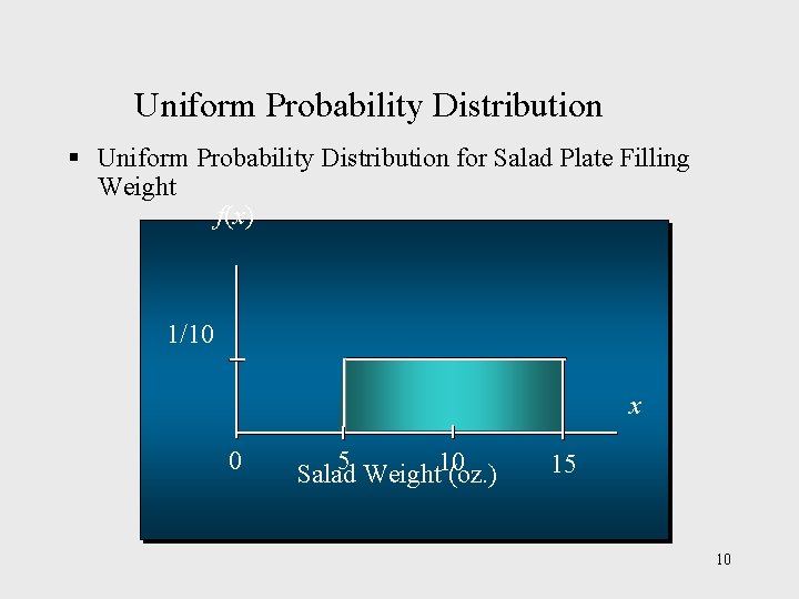
Uniform Probability Distribution § Uniform Probability Distribution for Salad Plate Filling Weight f(x) 1/10 x 0 5 Salad Weight 10 (oz. ) 15 10
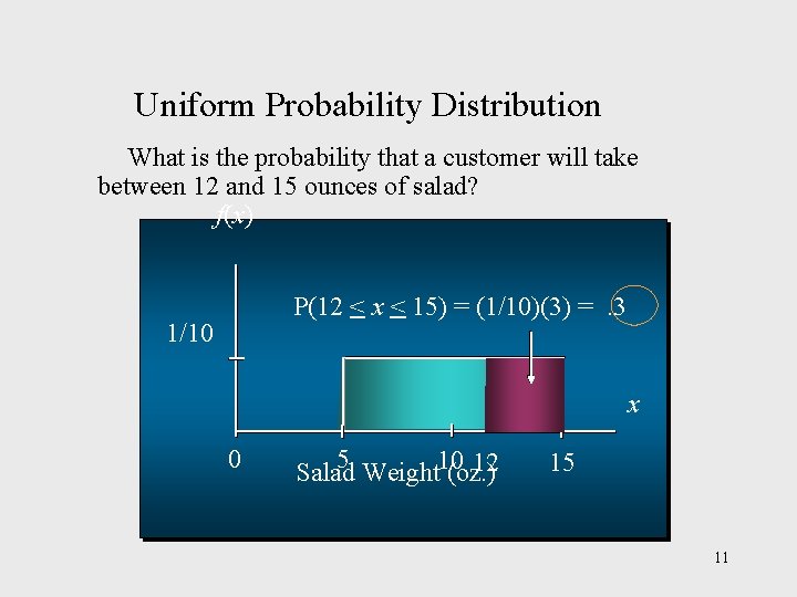
Uniform Probability Distribution What is the probability that a customer will take between 12 and 15 ounces of salad? f(x) P(12 < x < 15) = (1/10)(3) =. 3 1/10 x 0 5 12 Salad Weight 10 (oz. ) 15 11
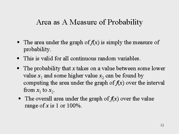
Area as A Measure of Probability § The area under the graph of f(x) is simply the measure of probability. § This is valid for all continuous random variables. § The probability that x takes on a value between some lower value x 1 and some higher value x 2 can be found by computing the area under the graph of f(x) over the interval from x 1 to x 2. § The overall area under the graph of f(x) over the value range of x is 1 or 100%. 12
Normal Probability Distribution § The normal probability distribution is the most important distribution for describing a continuous random variable. § It is widely used in statistical inference. § It has been used in describing a wide variety of real-life applications including: • Heights of people • Test scores • Rainfall amounts • Scientific measurements 13
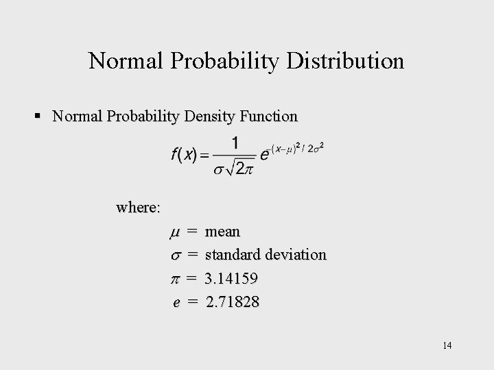
Normal Probability Distribution § Normal Probability Density Function where: = = = e = mean standard deviation 3. 14159 2. 71828 14
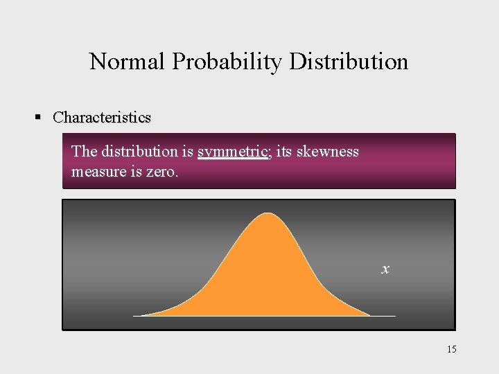
Normal Probability Distribution § Characteristics The distribution is symmetric; its skewness measure is zero. x 15
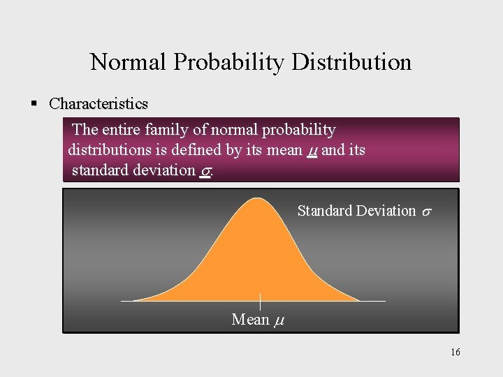
Normal Probability Distribution § Characteristics The entire family of normal probability distributions is defined by its mean and its standard deviation . Standard Deviation Mean 16
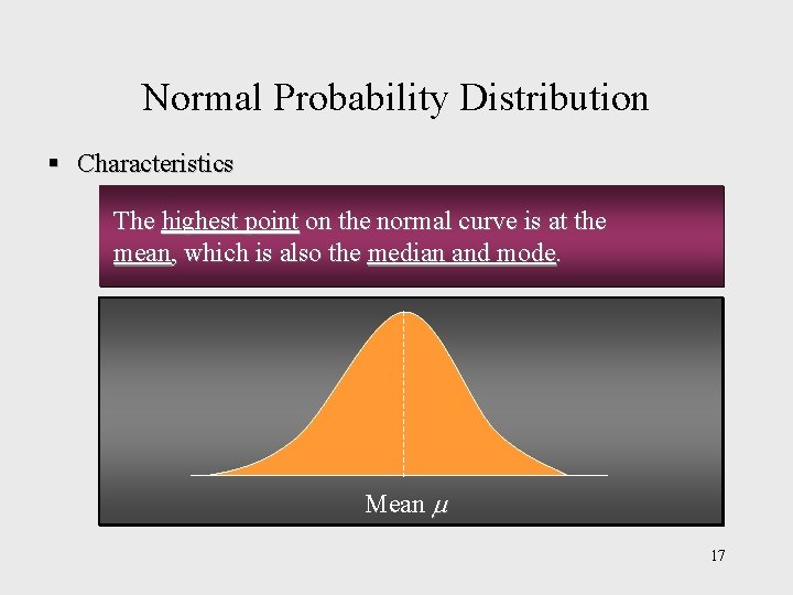
Normal Probability Distribution § Characteristics The highest point on the normal curve is at the mean, which is also the median and mode. Mean 17
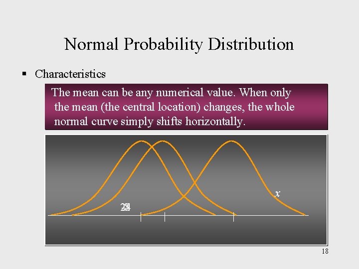
Normal Probability Distribution § Characteristics The mean can be any numerical value. When only the mean (the central location) changes, the whole normal curve simply shifts horizontally. x 24 -8 0 18
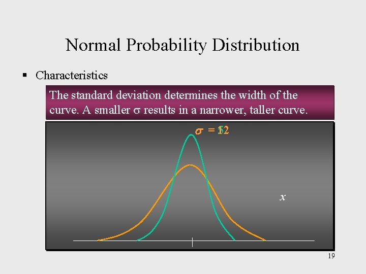
Normal Probability Distribution § Characteristics The standard deviation determines the width of the curve. A smaller results in a narrower, taller curve. s = 12 5 x 19
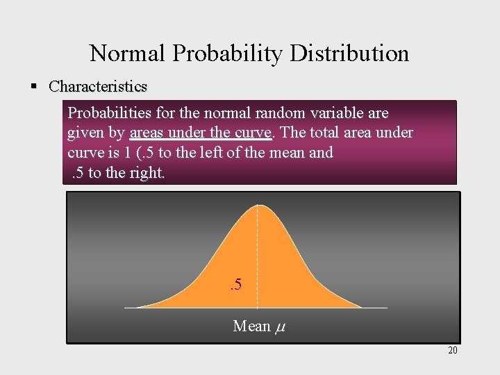
Normal Probability Distribution § Characteristics Probabilities for the normal random variable are given by areas under the curve. The total area under curve is 1 (. 5 to the left of the mean and. 5 to the right. . 5 Mean 20
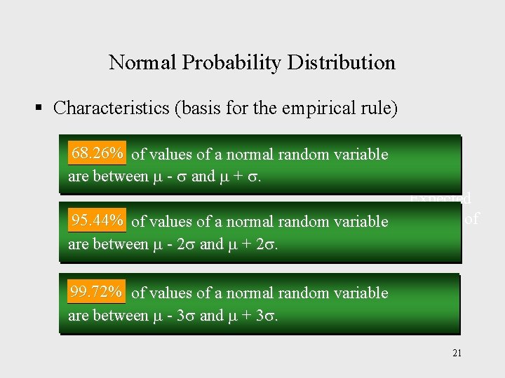
Normal Probability Distribution § Characteristics (basis for the empirical rule) 68. 26% of values of a normal random variable are between - and + . 95. 44% of values of a normal random variable are between - 2 and + 2. Expected number of correct answers 99. 72% of values of a normal random variable are between - 3 and + 3. 21
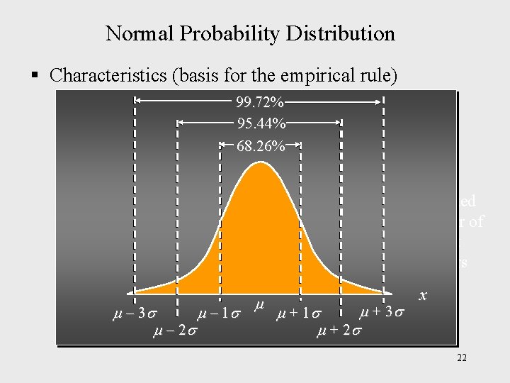
Normal Probability Distribution § Characteristics (basis for the empirical rule) 99. 72% 95. 44% 68. 26% Expected number of correct answers + 3 – 1 + 1 – 2 + 2 x 22
Standard Normal Probability Distribution § Characteristics (basis for the empirical rule) A normally distributed random variable with a mean of 0 and a standard deviation of 1 is said to have a standard normal probability distribution. Any other normal distribution can be Expected number of converted to the standard normal distribution. correct answers 23
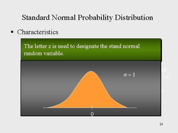
Standard Normal Probability Distribution § Characteristics The letter z is used to designate the stand normal random variable. =1 Expected number of correct answers 0 24
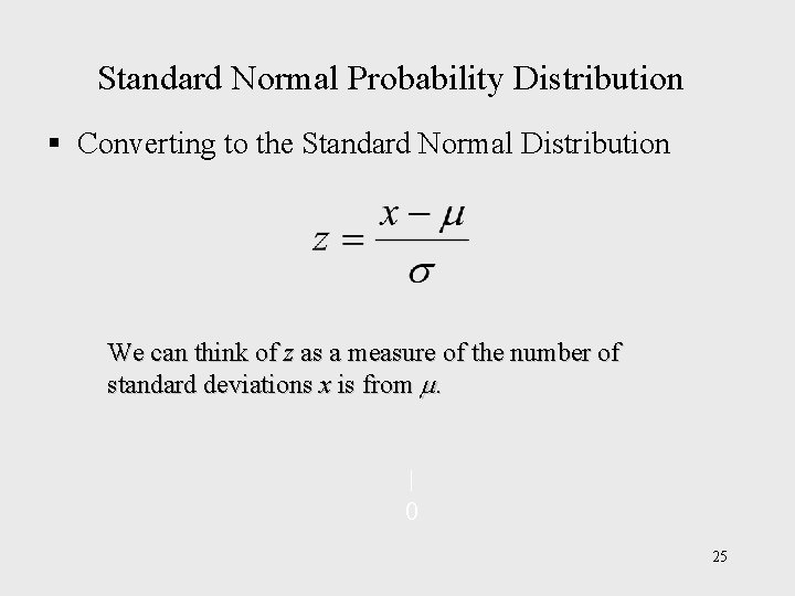
Standard Normal Probability Distribution § Converting to the Standard Normal Distribution We can think of z as a measure of the number of standard deviations x is from . 0 25
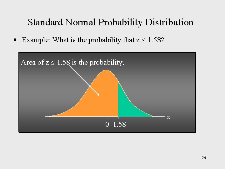
Standard Normal Probability Distribution § Example: What is the probability that z 1. 58? Area of z 1. 58 is the probability. 0 1. 58 z 26
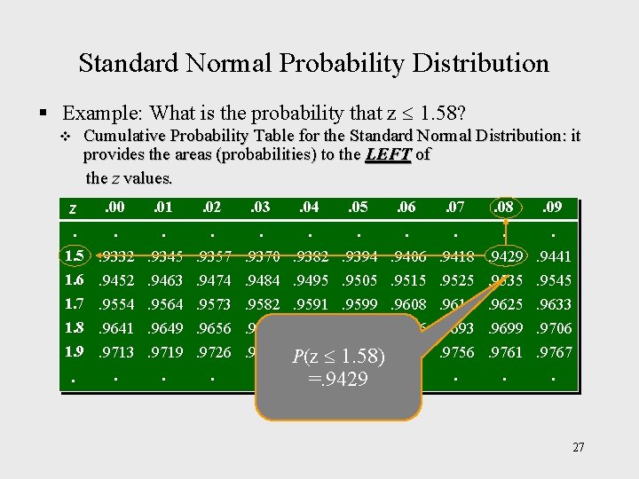
Standard Normal Probability Distribution § Example: What is the probability that z 1. 58? v z. Cumulative Probability Table for the Standard Normal Distribution: it provides the areas (probabilities) to the LEFT of the z values. . 00 . 01 . 02 . 03 . 04 . 05 . 06 . 07 . 08 . 09 . . 1. 5. 9332. 9345. 9357. 9370. 9382 1. 6. 9452. 9463. 9474. 9484. 9495 1. 7. 9554. 9564. 9573. 9582. 9591 1. 8. 9641. 9649. 9656. 9664. 9671 . 9394. 9406. 9418. 9429. 9441. 9505. 9515. 9525. 9535. 9545. 9599. 9608. 9616. 9625. 9633. 9678. 9686. 9693. 9699. 9706 1. 9. 9713. 9719. 9726. 9732 P(z. 9738 1. 58). 9744. 9750. 9756. 9761. 9767. . . =. 9429. . . 27
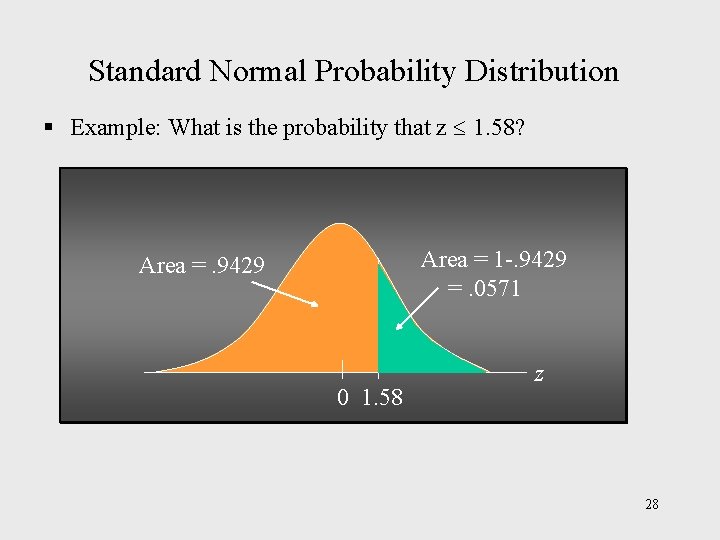
Standard Normal Probability Distribution § Example: What is the probability that z 1. 58? Area = 1 -. 9429 =. 0571 Area =. 9429 0 1. 58 z 28
Standard Normal Probability Distribution § Example: Computer Prices The average price of personal computers manufactured by Company APO is $1, 000 with a standard deviation of $150. Furthermore, it is known that the computer prices manufactured by APO are normally distributed. a. What is the probability that a randomly selected computer will have a price of at least $1125? P(x 1125) = ? 29
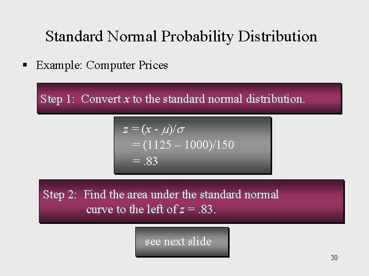
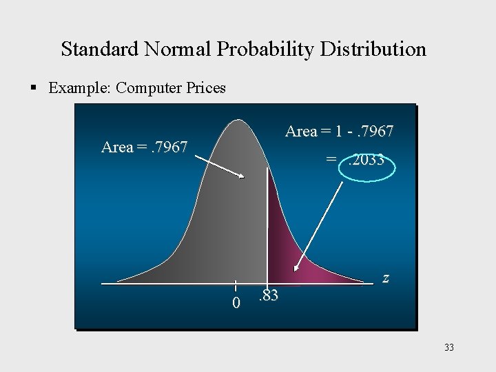
Standard Normal Probability Distribution § Example: Computer Prices Step 1: Convert x to the standard normal distribution. z = (x - )/ = (1125 – 1000)/150 =. 83 Step 2: Find the area under the standard normal curve to the left of z =. 83. see next slide 30
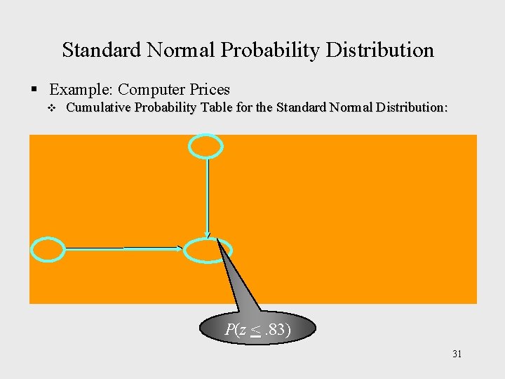
Standard Normal Probability Distribution § Example: Computer Prices v Cumulative Probability Table for the Standard Normal Distribution: P(z <. 83) 31
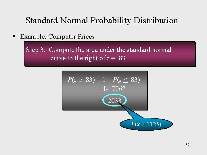
Standard Normal Probability Distribution § Example: Computer Prices Step 3: Compute the area under the standard normal curve to the right of z =. 83. P(z . 83) = 1 – P(z <. 83) = 1 -. 7967 =. 2033 P(x 1125) 32
Standard Normal Probability Distribution § Example: Computer Prices Area = 1 -. 7967 Area =. 7967 =. 2033 0 . 83 z 33
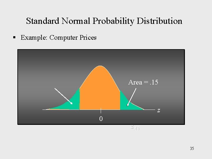
Standard Normal Probability Distribution § Example: Computer Prices b. To attract buyers like college students, Company APO decides to provide promotions on the cheaper computers. What is the maximum price such that only 15% of all the computers are eligible for a promotion sale? -----------------------------------(Hint: Given a probability (area), we can use the standard normal table in an inverse fashion to find the corresponding z value. ) 34
Standard Normal Probability Distribution § Example: Computer Prices Area =. 15 z 0 z. 15. 85 35
Standard Normal Probability Distribution § Example: Computer Prices Step 1: Determine whether the z value is negative or positive. The question is asking for the maximum computer price such that the cheapest computers (15% of all the computers) can enjoy a promotion sale. It is translated as: P(x <pricemax) =. 15 Therefore, the z value should be negative and it cuts off an area of. 15 in the left tail of the standard normal distribution. 36
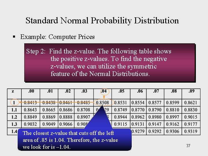
Standard Normal Probability Distribution § Example: Computer Prices Step 2: Find the z-value. The following table shows the positive z-values. To find the negative z-values, we can utilize the symmetric feature of the Normal Distributions. The closest z-value that cuts off the left area of. 85 is 1. 04. Therefore, the z-value we look for is – 1. 04. 37
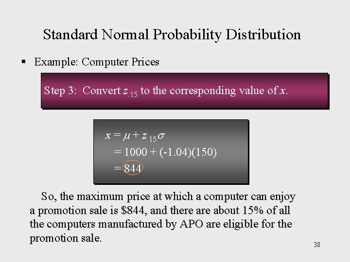
Standard Normal Probability Distribution § Example: Computer Prices Step 3: Convert z. 15 to the corresponding value of x. x = + z. 15 = 1000 + (-1. 04)(150) = 844 So, the maximum price at which a computer can enjoy a promotion sale is $844, and there about 15% of all the computers manufactured by APO are eligible for the promotion sale. 38
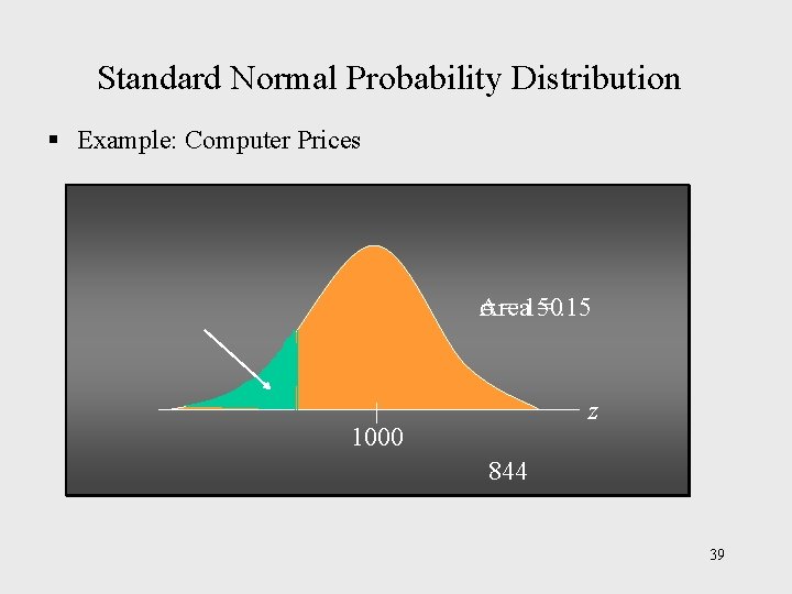
Standard Normal Probability Distribution § Example: Computer Prices = 150 Area =. 15 z 1000 844 39
- Slides: 39