Chapter 6 Binomial Probability Distributions December 21 In

Chapter 6: Binomial Probability Distributions December 21

In Chapter 6: 6. 1 Binomial Random Variables 6. 2 Calculating Binomial Probabilities 6. 3 Cumulative Probabilities 6. 4 Probability Calculators 6. 5 Expected Value and Variance of Binomial Random Variables 6. 6 Using the Binomial Distribution to Help Make Judgments

§ 6. 1 Binomial Random Variables • Binomial = a family of discrete random variables • Binomial random variable ≡ the random number of successes in n independent Bernoulli trials (a Bernoulli trials has two possible outcomes: “success” or “failure” • Binomials random variables have two parameters n number of trials p probability of success of each trial

Binomial Example • Consider the random number of successful treatments when treating four patients • Suppose the probability of success in each instance is 75% • The random number of successes can vary from 0 to 4 • The random number of successes is a binomial with parameters n = 4 and p = 0. 75 • Notation: Let X ~b(n, p) represent a binomial random variable with parameters n and p. The illustration variable is X ~ b(4, . 75)

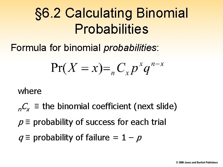
§ 6. 2 Calculating Binomial Probabilities Formula for binomial probabilities: where n. C x ≡ the binomial coefficient (next slide) p ≡ probability of success for each trial q ≡ probability of failure = 1 – p

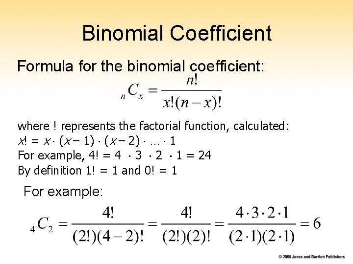
Binomial Coefficient Formula for the binomial coefficient: where ! represents the factorial function, calculated: x! = x (x – 1) (x – 2) … 1 For example, 4! = 4 3 2 1 = 24 By definition 1! = 1 and 0! = 1 For example:

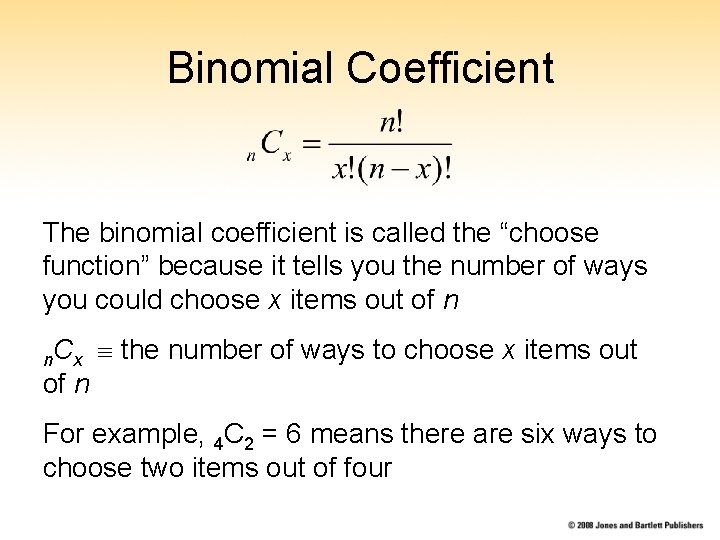
Binomial Coefficient The binomial coefficient is called the “choose function” because it tells you the number of ways you could choose x items out of n n. C x the number of ways to choose x items out of n For example, 4 C 2 = 6 means there are six ways to choose two items out of four

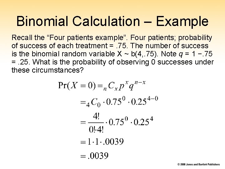
Binomial Calculation – Example Recall the “Four patients example”. Four patients; probability of success of each treatment =. 75. The number of success is the binomial random variable X ~ b(4, . 75). Note q = 1 −. 75 =. 25. What is the probability of observing 0 successes under these circumstances?

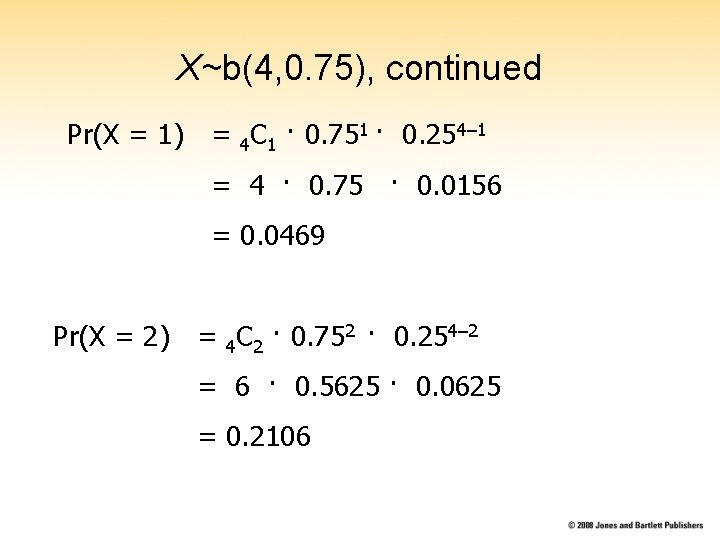
X~b(4, 0. 75), continued Pr(X = 1) = 4 C 1 · 0. 751 · 0. 254– 1 = 4 · 0. 75 · 0. 0156 = 0. 0469 Pr(X = 2) = 4 C 2 · 0. 752 · 0. 254– 2 = 6 · 0. 5625 · 0. 0625 = 0. 2106

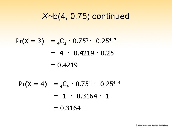
X~b(4, 0. 75) continued Pr(X = 3) = 4 C 3 · 0. 753 · 0. 254– 3 = 4 · 0. 4219 · 0. 25 = 0. 4219 Pr(X = 4) = 4 C 4 · 0. 754 · 0. 254– 4 = 1 · 0. 3164 · 1 = 0. 3164

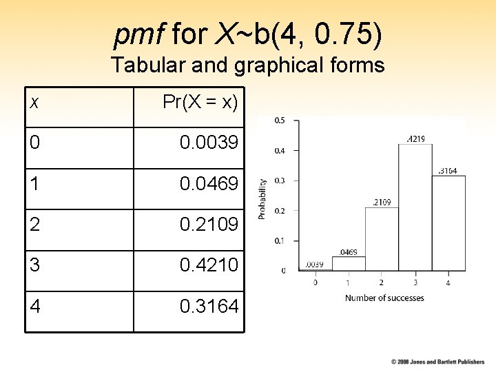
pmf for X~b(4, 0. 75) Tabular and graphical forms x Pr(X = x) 0 0. 0039 1 0. 0469 2 0. 2109 3 0. 4210 4 0. 3164

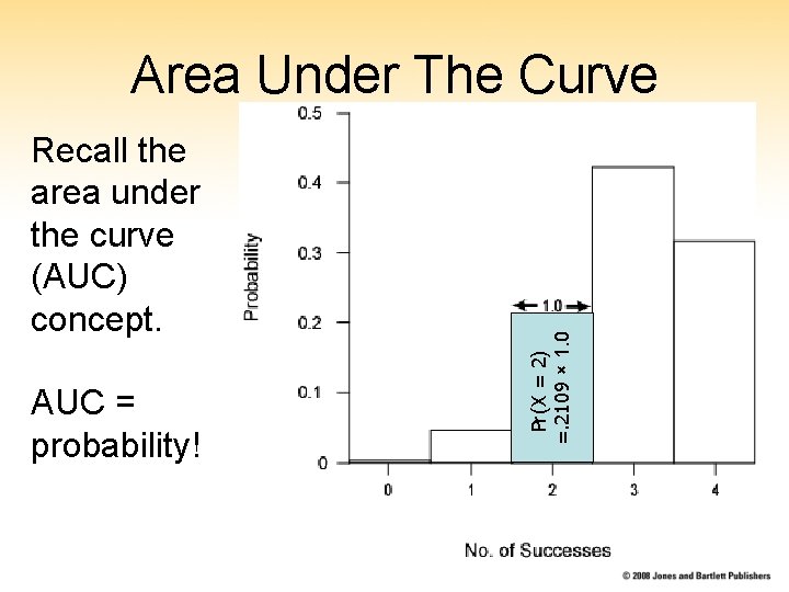
Recall the area under the curve (AUC) concept. AUC = probability! Pr(X = 2) =. 2109 × 1. 0 Area Under The Curve

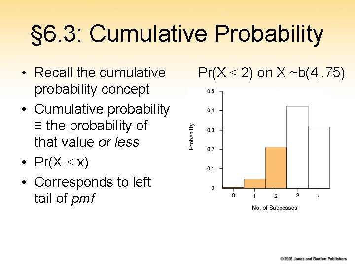
§ 6. 3: Cumulative Probability • Recall the cumulative probability concept • Cumulative probability ≡ the probability of that value or less • Pr(X x) • Corresponds to left tail of pmf Pr(X 2) on X ~b(4, . 75)

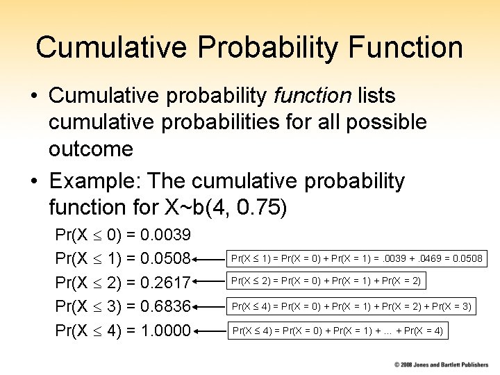
Cumulative Probability Function • Cumulative probability function lists cumulative probabilities for all possible outcome • Example: The cumulative probability function for X~b(4, 0. 75) Pr(X 0) = 0. 0039 Pr(X 1) = 0. 0508 Pr(X 2) = 0. 2617 Pr(X 3) = 0. 6836 Pr(X 4) = 1. 0000 Pr(X 1) = Pr(X = 0) + Pr(X = 1) =. 0039 +. 0469 = 0. 0508 Pr(X 2) = Pr(X = 0) + Pr(X = 1) + Pr(X = 2) Pr(X 4) = Pr(X = 0) + Pr(X = 1) + Pr(X = 2) + Pr(X = 3) Pr(X 4) = Pr(X = 0) + Pr(X = 1) + … + Pr(X = 4)

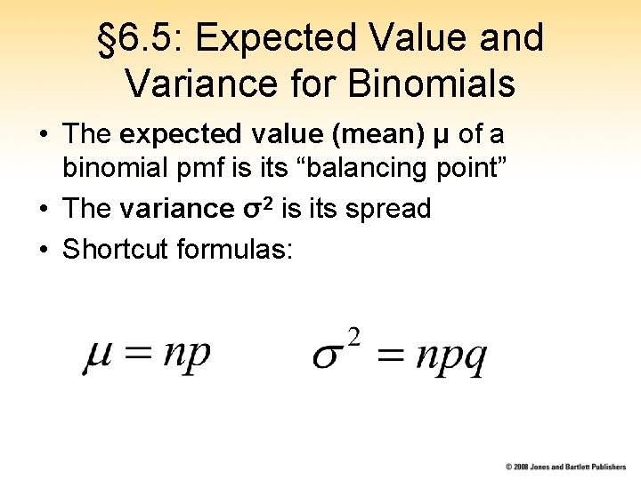
§ 6. 5: Expected Value and Variance for Binomials • The expected value (mean) μ of a binomial pmf is its “balancing point” • The variance σ2 is its spread • Shortcut formulas:

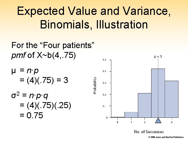
Expected Value and Variance, Binomials, Illustration For the “Four patients” pmf of X~b(4, . 75) μ = n∙p = (4)(. 75) = 3 σ2 = n∙p∙q = (4)(. 75)(. 25) = 0. 75

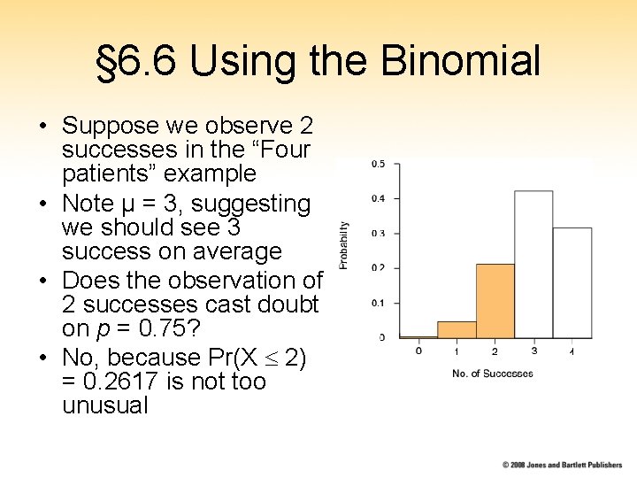
§ 6. 6 Using the Binomial • Suppose we observe 2 successes in the “Four patients” example • Note μ = 3, suggesting we should see 3 success on average • Does the observation of 2 successes cast doubt on p = 0. 75? • No, because Pr(X 2) = 0. 2617 is not too unusual

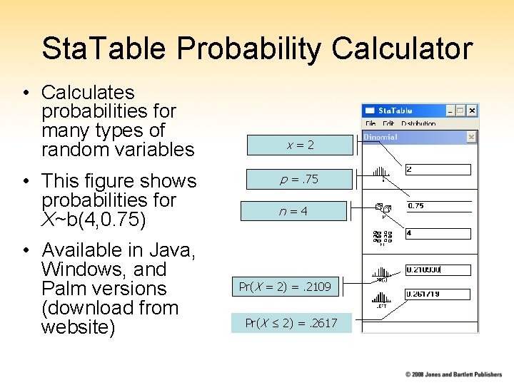
Sta. Table Probability Calculator • Calculates probabilities for many types of random variables • This figure shows probabilities for X~b(4, 0. 75) • Available in Java, Windows, and Palm versions (download from website) x=2 p =. 75 n=4 Pr(X = 2) =. 2109 Pr(X ≤ 2) =. 2617