Chapter 6 Backpropagation Nets Architecture at least one

Chapter 6: Backpropagation Nets • Architecture: at least one layer of non-linear hidden units • Learning: supervised, error driven, generalized delta rule • Derivation of the weight update formula (with gradient descent approach) • Practical considerations • Variations of BP nets • Applications

Architecture of BP Nets • Multi-layer, feed-forward network – Must have at least one hidden layer – Hidden units must be non-linear units (usually with sigmoid activation functions) – Fully connected between units in two consecutive layers, but no connection between units within one layer. • For a net with only one hidden layer, each hidden unit z_j receives input from all input units x_i and sends output to all output units y_k x 1 v_1 p z 1 w_1 k Yk v_n 1 xn v_np non-linear units zp w_2 k

– Additional notations: (nets with one hidden layer) x = (x_1, . . . x_n): input vector z = (z_1, . . . z_p): hidden vector (after x applied on input layer) y = (y_1, . . . y_m): output vector (computation result) delta_k: error term on Y_k • Used to update weights w_jk • Backpropagated to z_j delta_j: error term on Z_j weighted input • Used to update weights v_ij z_inj: = v_0 j + Sum(x_i * v_ij): input to hidden unit Z_j y_inj: = w_0 k + Sum(z_j * w_jk): input to output unit Y_k bias x_i v_ij 1 1 v_0 j w_0 k z_j w_jk y_k

– Forward computing: • Apply an input vector x to input units • Computing activation/output vector z on hidden layer • Computing the output vector y on output layer y is the result of the computation. • The net is said to be a map from input x to output y – Theoretically nets of such architecture able to approximate any L 2 functions (all integral functions, including almost all commonly used math functions) to any given degree of accuracy, provided there are sufficient many hidden units – Question: How to get these weights so that the mapping is what you want

Learning for BP Nets – Update of weights in W (between output and hidden layers): delta rule as in a single layer net – Delta rule is not applicable to updating weights in V (between input and hidden layers) because we don’t know the target values for hidden units z_1, . . . z_p – Solution: Propagating errors at output units to hidden units, these computed errors on hidden units drives the update of weights in V (again by delta rule), thus called error BACKPROPAGATION learning – How to compute errors on hidden units is the key – Error backpropagation can be continued downward if the net has more than one hidden layer.

BP Learning Algorithm step 0: initialize the weights (W and V), including biases, to small random numbers step 1: while stop condition is false do steps 2 – 9 step 2: for each training sample x: t do steps 3 – 8 /* Feed-forward phase (computing output vector y) */ step 3: apply vector x to input layer step 4: compute input and output for each hidden unit Z_j z_inj : = v_0 j + Sum(x_i * v_ij); z_j : = f(z_inj); step 5: compute input and output for each output unit Y_k y_ink : = w_0 k + Sum(v_j * w_jk); y_k : = f(y_ink);

/* Error backpropagation phase */ step 6: for each output unit Y_k delta_k : = (t_k – y_k)*f’(y_ink) /* error term */ delta_w_jk : = alpha*delta_k*z_j /* weight change */ step 7: For each hidden unit Z_j delta_inj : = Sum(delta_k * w_jk) /* erro BP */ delta_j : = delta_inj * f’(z_inj) /*error term */ delta_v_ij : = alpha*delta_j*x_i /* weight change */ step 8: Update weights (incl. biases) w_jk : = w_jk + delta_w_jk for all j, k; v_ij : = v_ij + delta_v_ij for all i, j; step 9: test stop condition

Notes on BP learning: – The error term for a hidden unit z_j is the weighted sum of error terms delta_k of all output units Y_k delta_inj : = Sum(delta_k * w_jk) times the derivative of its own output (f’(z_inj) In other words, delta_inj plays the same role for hidden units v_j as (t_k – y_k) for output units y_k – Sigmoid function can be either binary or bipolar – For multiple hidden layers: repeat step 7 (downward) – Stop condition: • Total output error E = Sum(t_k – y_k)^2 falls into the given acceptable error range • E changes very little for quite awhile • Maximum time (or number of epochs) is reached.

Derivation of BP Learning Rule • Objective of BP learning: minimize the mean squared output error over all training samples For clarity, the derivation is for error of one sample • Approach: gradient descent. Gradient given the direction and magnitude of change of f w. r. t its arguments • For a function of single argument Gradient descent requires that x changes in the opposite direction of the gradient, i. e. , . Then since for small we have y monotonically decreases

• For a multi-variable function (e. g. , our error function E) Gradient descent requires each argument opposite direction of the corresponding changes in the Then because we have • Gradient descent guarantees that E monotonically decreases, and • Chain rule of derivatives is used for deriving partial derivatives

Update W, the weights of the output layer For a particular weight (from units to ) The last equality comes from the fact that only one of the terms in , namely involves This is the update rule in Step 6 of the algorithm

Update V, the weights of the hidden layer For a particular weight (from unit to ) The last equality comes from the fact that only one of the terms in , namely involves

This is the update rule in Step 7 of the algorithm

Strengths of BP Nets • Great representation power – Any L 2 function can be represented by a BP net (multi-layer feed-forward net with non-linear hidden units) – Many such functions can be learned by BP learning (gradient descent approach) • Wide applicability of BP learning – Only requires that a good set of training samples is available) – Does not require substantial prior knowledge or deep understanding of the domain itself (ill structured problems) – Tolerates noise and missing data in training samples (graceful degrading) • Easy to implement the core of the learning algorithm • Good generalization power – Accurate results for inputs outside the training set

Deficiencies of BP Nets • Learning often takes a long time to converge – Complex functions often need hundreds or thousands of epochs • The net is essentially a black box – If may provide a desired mapping between input and output vectors (x, y) but does not have the information of why a particular x is mapped to a particular y. – It thus cannot provide an intuitive (e. g. , causal) explanation for the computed result. – This is because the hidden units and the learned weights do not have a semantics. What can be learned are operational parameters, not general, abstract knowledge of a domain • Gradient descent approach only guarantees to reduce the total error to a local minimum. (E may be be reduced to zero) – Cannot escape from the local minimum error state – Not every function that is representable can be learned

– How bad: depends on the shape of the error surface. Too many valleys/wells will make it easy to be trapped in local minima – Possible remedies: • Try nets with different # of hidden layers and hidden units (they may lead to different error surfaces, some might be better than others) • Try different initial weights (different starting points on the surface) • Forced escape from local minima by random perturbation (e. g. , simulated annealing) • Generalization is not guaranteed even if the error is reduced to zero – Over-fitting/over-training problem: trained net fits the training samples perfectly (E reduced to 0) but it does not give accurate outputs for inputs not in the training set • Unlike many statistical methods, there is no theoretically wellfounded way to assess the quality of BP learning – What is the confidence level one can have for a trained BP net, with the final E (which not or may not be close to zero)

• Network paralysis with sigmoid activation function – Saturation regions: |x| >> 1 – Input to an unit may fall into a saturation region when some of its incoming weights become very large during learning. Consequently, weights stop to change no matter how hard you try. – Possible remedies: • Use non-saturating activation functions • Periodically normalize all weights

• The learning (accuracy, speed, and generalization) is highly dependent of a set of learning parameters – Initial weights, learning rate, # of hidden layers and # of units. . . – Most of them can only be determined empirically (via experiments)

Practical Considerations • A good BP net requires more than the core of the learning algorithms. Many parameters must be carefully selected to ensure a good performance. • Although the deficiencies of BP nets cannot be completely cured, some of them can be eased by some practical means. • Initial weights (and biases) – Random, [-0. 05, 0. 05], [-0. 1, 0. 1], [-1, 1] – Normalize weights for hidden layer (v_ij) (Nguyen-Widrow) • Random assign v_ij for all hidden units V_j • For each V_j, normalize its weight by where is the normalization factor • Avoid bias in weight initialization:

• Training samples: – Quality and quantity of training samples determines the quality of learning results – Samples must be good representatives of the problem space • Random sampling • Proportional sampling (with prior knowledge of the problem space) – # of training patterns needed: • There is no theoretically idea number. Following is a rule of thumb • W: total # of weights to be trained (depends on net structure) e: desired classification error rate • If we have P = W/e training patterns, and we can train a net to correctly classify (1 – e/2)P of them, • Then this net would (in a statistical sense) be able to correctly classify a fraction of 1 – e input patterns drawn from the sample space • Example: W = 80, e = 0. 1, P = 800. If we can successfully train the network to correctly classify (1 – 0. 1/2)*800 = 760 of the samples, we would believe that the net will work correctly 90% of time with other input.

• Data representation: – Binary vs bipolar • Bipolar representation uses training samples more efficiently no learning will occur when with binary rep. • # of patterns can be represented n input units: binary: 2^n bipolar: 2^(n-1) if no biases used, this is due to (anti)symmetry (if the net outputs y for input x, it will output –y for input –x) – Real value data • Input units: real value units (may subject to normalization) • Hidden units are sigmoid • Activation function for output units: often linear (even identity) e. g. , • Training may be much slower than with binary/bipolar data (some use binary encoding of real values)

• How many hidden layers and hidden units per layer: – Theoretically, one hidden layer (possibly with many hidden units) is sufficient for any L 2 functions – There is no theoretical results on minimum necessary # of hidden units (either problem dependent or independent) – Practical rule of thumb: • n = # of input units; p = # of hidden units • For binary/bipolar data: p = 2 n • For real data: p >> 2 n – Multiple hidden layers with fewer units may be trained faster for similar quality in some applications

• Over-training/over-fitting – Trained net fits very well with the training samples (total error ), but not with new input patterns – Over-training may become serious if • Training samples were not obtained properly • Training samples have noise – Control over-training for better generalization • Cross-validation: dividing the samples into two sets - 90% into training set: used to train the network - 10% into test set: used to validate training results periodically test the trained net with test samples, stop training when test results start to deteriorating. • Stop training early (before ) • Add noise to training samples: x: t becomes x+noise: t (for binary/bipolar: flip randomly selected input units)

Variations of BP nets • Adding momentum term (to speedup learning) – Weights update at time t+1 contains the momentum of the previous updates, e. g. , an exponentially weighted sum of all previous updates – Avoid sudden change of directions of weight update (smoothing the learning process) – Error is no longer monotonically decreasing • Batch mode of weight updates – Weight update once per each epoch – Smoothing the training sample outliers – Learning independent of the order of sample presentations – Usually slower than in sequential mode

• Variations on learning rate a – Give known underrepresented samples higher rates – Find the maximum safe step size at each stage of learning (to avoid overshoot the minimum E when increasing a) – Adaptive learning rate (delta-bar-delta method) • Each weight w_jk has its own rate a_jk • If remains in the same direction, increase a_jk (E has a smooth curve in the vicinity of current W) • If changes the direction, decrease a_jk (E has a rough curve in the vicinity of current W)

– delta-bar-delta also involves momentum term (of a) – Experimental comparison • Training for XOR problem (batch mode) • 25 simulations: success if E averaged over 50 consecutive epochs is less than 0. 04 • results method simulations success Mean epochs BP 25 24 16, 859. 8 BP with momentum 25 25 2, 056. 3 BP with deltabar-delta 25 22 447. 3

• Other activation functions – Change the range of the logistic function from (0, 1) to (a, b)

– Change the slope of the logistic function • Larger slope: quicker to move to saturation regions; faster convergence • Smaller slope: slow to move to saturation regions, allows refined weight adjustment • s thus has a effect similar to the learning rate a (but more drastic) – Adaptive slope (each node has a learned slope)

– Another sigmoid function with slower saturation speed the derivative of logistic function – A non-saturating function (also differentiable)

– Non-sigmoid activation function Radial based function: it has a center c.

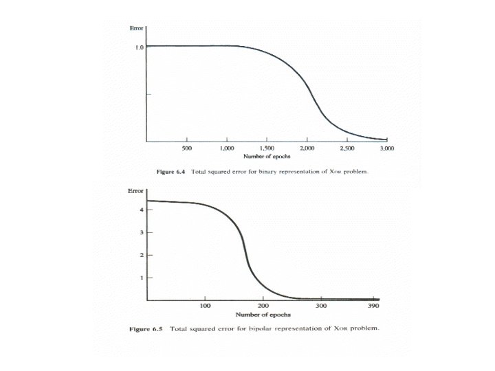
Applications of BP Nets • A simple example: Learning XOR – Initial weights and other parameters • weights: random numbers in [-0. 5, 0. 5] • hidden units: single layer of 4 units (A 2 -4 -1 net) • biases used; • learning rate: 0. 02 – Variations tested • binary vs. bipolar representation • different stop criteria • normalizing initial weights (Nguyen-Widrow) – Bipolar is faster than binary • convergence: ~3000 epochs for binary, ~400 for bipolar • Why?

– Relaxing acceptable error range may speed up convergence • is an asymptotic limits of sigmoid function, • When an output approaches , it falls in a saturation region • Use – Normalizing initial weights may also help Random Nguyen-Widrow Binary 2, 891 1, 935 Bipolar 387 224 Bipolar with 264 127

• Data compression – Autoassociation of patterns (vectors) with themselves using a small number of hidden units: • training samples: : x: x (x has dimension n) hidden units: m < n (A n-m-n net) V n W m n • If training is successful, applying any vector x on input units will generate the same x on output units • Pattern z on hidden layer becomes a compressed representation of x (with smaller dimension m < n) • Application: reducing transmission cost x n sender V m z z Communication channel m W receiver n x

– Example: compressing character bitmaps. • Each character is represented by a 7 by 9 pixel bitmap, or a binary vector of dimension 63 • 10 characters (A – J) are used in experiment • Error range: tight: 0. 1 (off: 0 – 0. 1; on: 0. 9 – 1. 0) loose: 0. 2 (off: 0 – 0. 2; on: 0. 8 – 1. 0) • Relationship between # hidden units, error range, and convergence rate (Fig. 6. 7, p. 304) – relaxing error range may speed up – increasing # hidden units (to a point) may speed up error range: 0. 1 hidden units: 10 # epochs 400+ error range: 0. 2 hidden units: 10 # epochs 200+ error range: 0. 1 hidden units: 20 # epochs 180+ error range: 0. 2 hidden units: 20 # epochs 90+ no noticeable speed up when # hidden units increases to beyond 22

• Other applications. – Medical diagnosis • Input: manifestation (symptoms, lab tests, etc. ) Output: possible disease(s) • Problems: – no causal relations can be established – hard to determine what should be included as inputs • Currently focus on more restricted diagnostic tasks – e. g. , predict prostate cancer or hepatitis B based on standard blood test – Process control • Input: environmental parameters Output: control parameters • Learn ill-structured control functions

– Stock market forecasting • Input: financial factors (CPI, interest rate, etc. ) and stock quotes of previous days (weeks) Output: forecast of stock prices or stock indices (e. g. , S&P 500) • Training samples: stock market data of past few years – Consumer credit evaluation • Input: personal financial information (income, debt, payment history, etc. ) • Output: credit rating – And many more – Key for successful application • Careful design of input vector (including all important features): some domain knowledge • Obtain good training samples: time and other cost

Summary of BP Nets • Architecture – Multi-layer, feed-forward (full connection between nodes in adjacent layers, no connection within a layer) – One or more hidden layers with non-linear activation function (most commonly used are sigmoid functions) • BP learning algorithm – Supervised learning (samples s: t) – Approach: gradient descent to reduce the total error (why it is also called generalized delta rule) – Error terms at output units error terms at hidden units (why it is called error BP) – Ways to speed up the learning process • Adding momentum terms • Adaptive learning rate (delta-bar-delta) – Generalization (cross-validation test)

• Strengths of BP learning – – Great representation power Wide practical applicability Easy to implement Good generalization power • Problems of BP learning – – – – Learning often takes a long time to converge The net is essentially a black box Gradient descent approach only guarantees a local minimum error Not every function that is representable can be learned Generalization is not guaranteed even if the error is reduced to zero No well-founded way to assess the quality of BP learning Network paralysis may occur (learning is stopped) Selection of learning parameters can only be done by trial-and-error – BP learning is non-incremental (to include new training samples, the network must be re-trained with all old and new samples)