Chapter 6 Artificial neural networks Introduction or how

Chapter 6 Artificial neural networks: Introduction, or how the brain works n The neuron as a simple computing element n The perceptron n Multilayer neural networks n Negnevitsky, Pearson Education, 2002 1

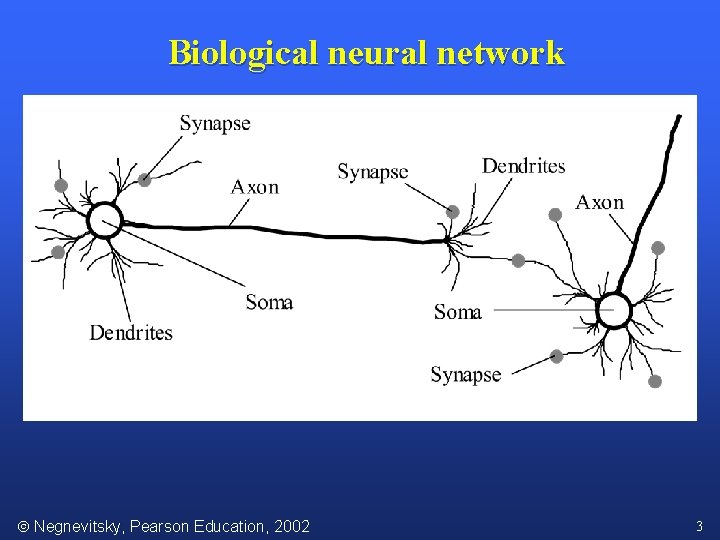
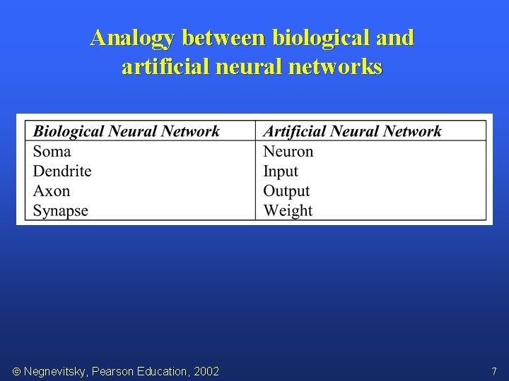
Neural Networks and the Brain n n n A neural network is a model of reasoning inspired by the human brain. The brain consists of a densely interconnected set of nerve cells, or basic information-processing units, called neurons. The human brain incorporates nearly 10 billion neurons and 60 trillion connections, synapses, between them. By using multiple neurons simultaneously, the brain can perform its functions much faster than the fastest computers in existence today. Each neuron has a very simple structure, but an army of such elements constitutes a tremendous processing power. A neuron consists of a cell body, soma, a number of fibers called dendrites, and a single long fiber called the axon. Negnevitsky, Pearson Education, 2002 2

Biological neural network Negnevitsky, Pearson Education, 2002 3

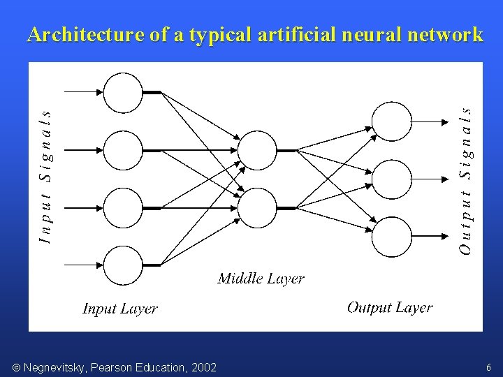
Architecture of a typical artificial neural network Negnevitsky, Pearson Education, 2002 6

Analogy between biological and artificial neural networks Negnevitsky, Pearson Education, 2002 7

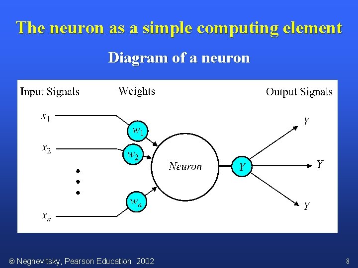
The neuron as a simple computing element Diagram of a neuron Negnevitsky, Pearson Education, 2002 8

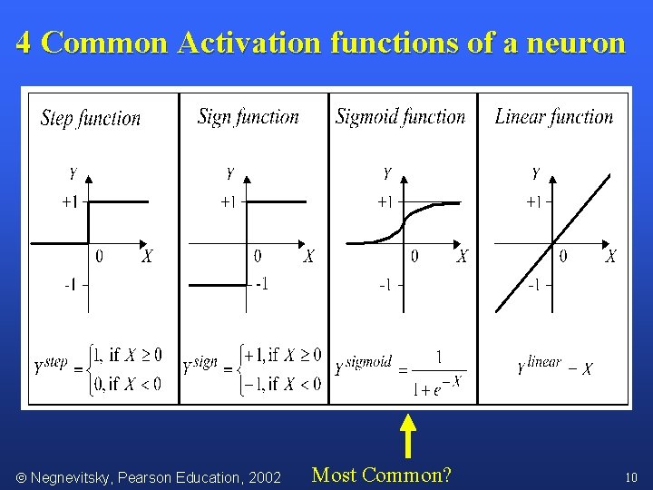
A Simple Activation Function – Sign Function n n The neuron computes the weighted sum of the input signals and compares the result with a threshold value, . If the net input is less than the threshold, the neuron output is – 1. if the net input is greater than or equal to the threshold, the neuron becomes activated and its output is +1. The neuron uses the following transfer or activation function: This type of activation function is called a sign function. (Mc. Culloch and Pitts 1943) Negnevitsky, Pearson Education, 2002 9

4 Common Activation functions of a neuron Negnevitsky, Pearson Education, 2002 Most Common? 10

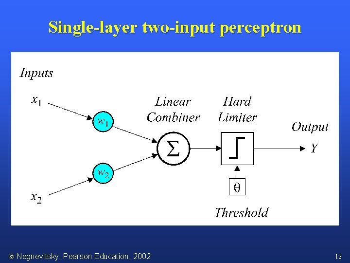
Can a single neuron learn a task? n Start off with earliest/ simplest n In 1958, Frank Rosenblatt introduced a training algorithm that provided the first procedure for training a simple ANN: a perceptron. n The perceptron is the simplest form of a neural network. It consists of a single neuron with adjustable synaptic weights and a hard limiter. Negnevitsky, Pearson Education, 2002 11

Single-layer two-input perceptron Negnevitsky, Pearson Education, 2002 12

The Perceptron The operation of Rosenblatt’s perceptron is based on the Mc. Culloch and Pitts neuron model. The model consists of a linear combiner followed by a hard limiter. n The weighted sum of the inputs is applied to the hard limiter, which produces an output equal to +1 if its input is positive and 1 if it is negative. n Negnevitsky, Pearson Education, 2002 13

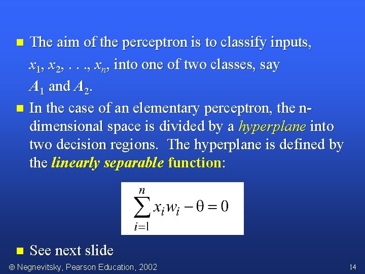
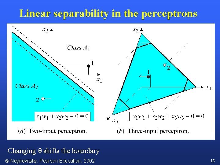
The aim of the perceptron is to classify inputs, x 1, x 2, . . . , xn, into one of two classes, say A 1 and A 2. n In the case of an elementary perceptron, the ndimensional space is divided by a hyperplane into two decision regions. The hyperplane is defined by the linearly separable function: n n See next slide Negnevitsky, Pearson Education, 2002 14

Linear separability in the perceptrons Changing θ shifts the boundary Negnevitsky, Pearson Education, 2002 15

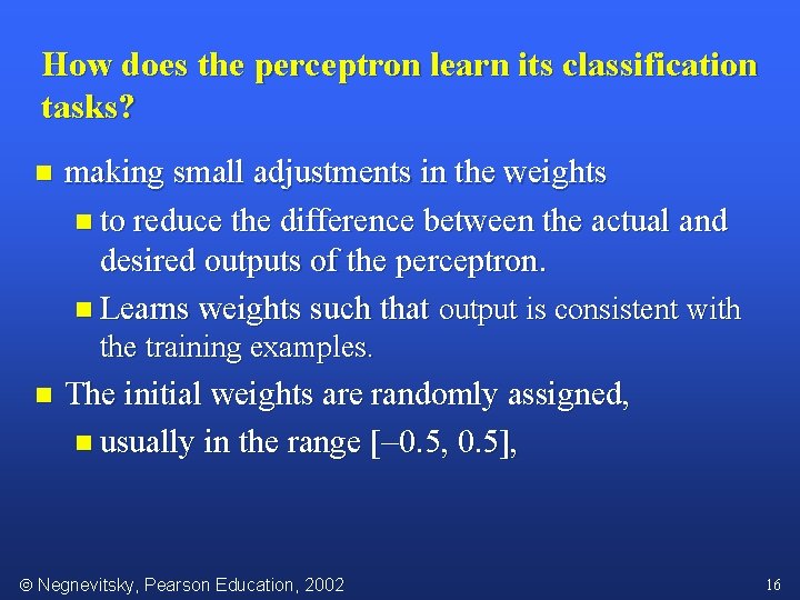
How does the perceptron learn its classification tasks? n making small adjustments in the weights n to reduce the difference between the actual and desired outputs of the perceptron. n Learns weights such that output is consistent with the training examples. n The initial weights are randomly assigned, n usually in the range [ 0. 5, 0. 5], Negnevitsky, Pearson Education, 2002 16

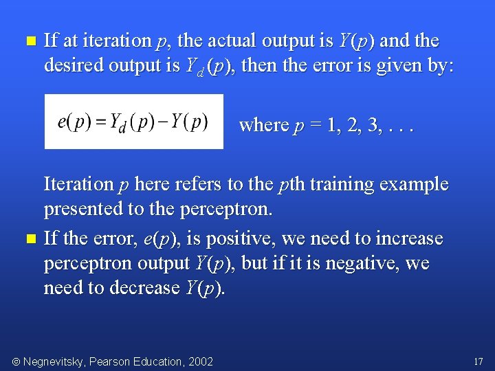
n If at iteration p, the actual output is Y(p) and the desired output is Yd (p), then the error is given by: where p = 1, 2, 3, . . . Iteration p here refers to the pth training example presented to the perceptron. n If the error, e(p), is positive, we need to increase perceptron output Y(p), but if it is negative, we need to decrease Y(p). Negnevitsky, Pearson Education, 2002 17

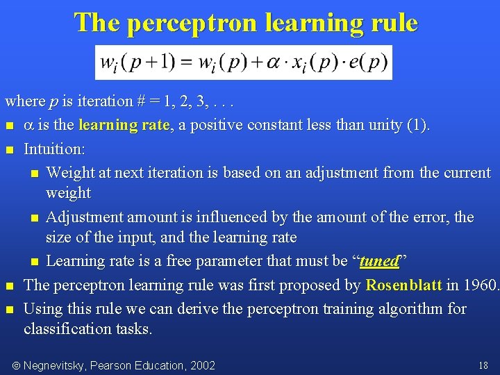
The perceptron learning rule where p is iteration # = 1, 2, 3, . . . n is the learning rate, a positive constant less than unity (1). n Intuition: n Weight at next iteration is based on an adjustment from the current weight n Adjustment amount is influenced by the amount of the error, the size of the input, and the learning rate n Learning rate is a free parameter that must be “tuned” n The perceptron learning rule was first proposed by Rosenblatt in 1960. n Using this rule we can derive the perceptron training algorithm for classification tasks. Negnevitsky, Pearson Education, 2002 18

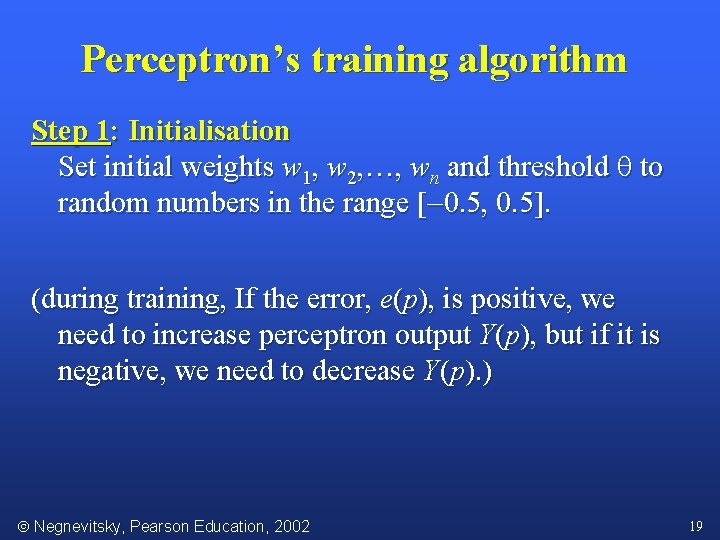
Perceptron’s training algorithm Step 1: Initialisation Set initial weights w 1, w 2, …, wn and threshold to random numbers in the range [ 0. 5, 0. 5]. (during training, If the error, e(p), is positive, we need to increase perceptron output Y(p), but if it is negative, we need to decrease Y(p). ) Negnevitsky, Pearson Education, 2002 19

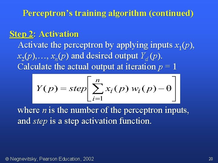
Perceptron’s training algorithm (continued) Step 2: Activation Activate the perceptron by applying inputs x 1(p), x 2(p), …, xn(p) and desired output Yd (p). Calculate the actual output at iteration p = 1 where n is the number of the perceptron inputs, and step is a step activation function. Negnevitsky, Pearson Education, 2002 20

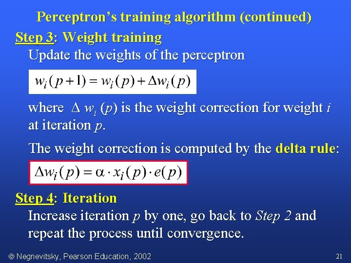
Perceptron’s training algorithm (continued) Step 3: Weight training Update the weights of the perceptron where Δ wi (p) is the weight correction for weight i at iteration p. The weight correction is computed by the delta rule: Step 4: Iteration Increase iteration p by one, go back to Step 2 and repeat the process until convergence. Negnevitsky, Pearson Education, 2002 21

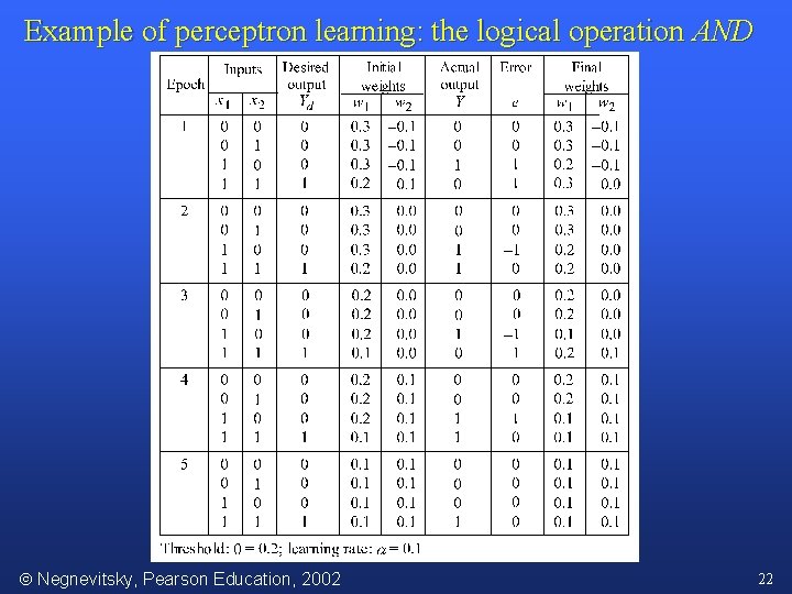
Example of perceptron learning: the logical operation AND Negnevitsky, Pearson Education, 2002 22

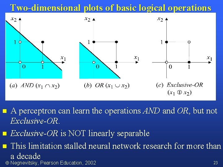
Two-dimensional plots of basic logical operations n n n A perceptron can learn the operations AND and OR, but not Exclusive-OR is NOT linearly separable This limitation stalled neural network research for more than a decade Negnevitsky, Pearson Education, 2002 23

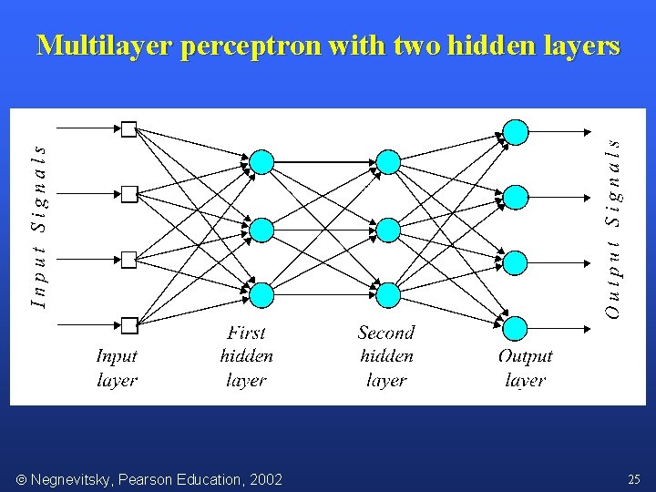
Multilayer neural networks A multilayer perceptron is a feedforward neural network with one or more hidden layers. n The network consists of an input layer of source neurons, at least one middle or hidden layer of computational neurons, and an output layer of computational neurons. n The input signals are propagated in a forward direction on a layer-by-layer basis. n Negnevitsky, Pearson Education, 2002 24

Multilayer perceptron with two hidden layers Negnevitsky, Pearson Education, 2002 25

Hidden Layer Detects features in the inputs – hidden patterns n With one hidden layer, can represent any continuous function of the inputs n With two hidden layers even discontinuous functions can be represented n Negnevitsky, Pearson Education, 2002 27

Back-propagation neural network Most popular of 100+ ANN learning algorithms n Learning in a multilayer network proceeds the same way as for a perceptron. n A training set of input patterns is presented to the network. n The network computes its output pattern, and if there is an error or in other words a difference between actual and desired output patterns the weights are adjusted to reduce this error. n The difference is in the number of weights and architecture … n Negnevitsky, Pearson Education, 2002 28

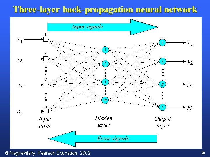
Back-propagation neural network n n In a back-propagation neural network, the learning algorithm has two phases: n a training input pattern is presented to the network input layer. n The network propagates the input pattern from layer to layer until the output pattern is generated by the output layer. n Activation function generally sigmoid n If this pattern is different from the desired output, an error is calculated and then propagated backwards through the network from the output layer to the input layer. The weights are modified as the error is propagated. See next slide for picture … Negnevitsky, Pearson Education, 2002 29

Three-layer back-propagation neural network Negnevitsky, Pearson Education, 2002 30

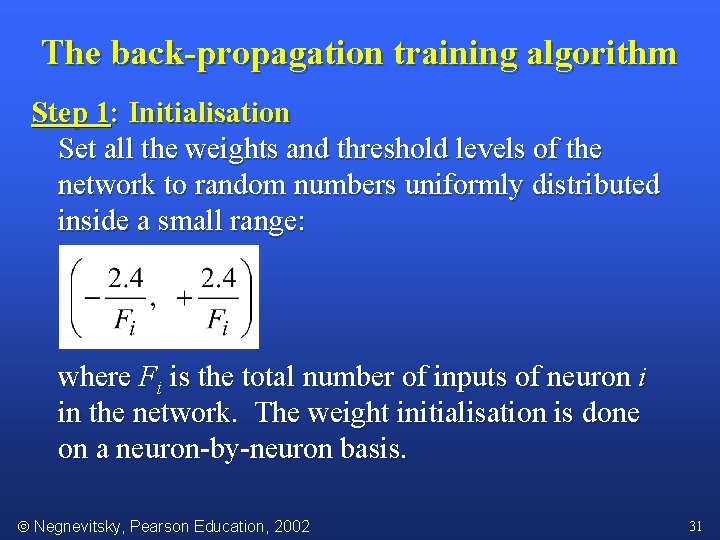
The back-propagation training algorithm Step 1: Initialisation Set all the weights and threshold levels of the network to random numbers uniformly distributed inside a small range: where Fi is the total number of inputs of neuron i in the network. The weight initialisation is done on a neuron-by-neuron basis. Negnevitsky, Pearson Education, 2002 31

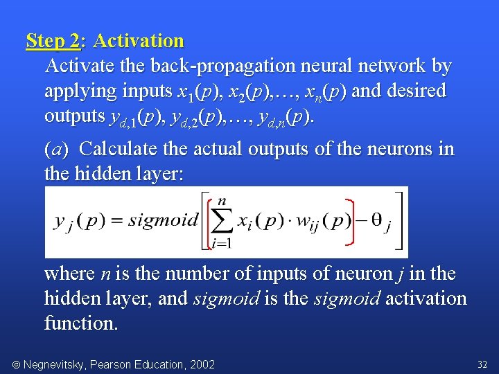
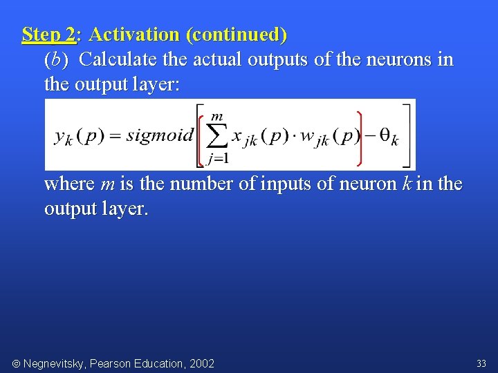
Step 2: Activation Activate the back-propagation neural network by applying inputs x 1(p), x 2(p), …, xn(p) and desired outputs yd, 1(p), yd, 2(p), …, yd, n(p). (a) Calculate the actual outputs of the neurons in the hidden layer: where n is the number of inputs of neuron j in the hidden layer, and sigmoid is the sigmoid activation function. Negnevitsky, Pearson Education, 2002 32

Step 2: Activation (continued) (b) Calculate the actual outputs of the neurons in the output layer: where m is the number of inputs of neuron k in the output layer. Negnevitsky, Pearson Education, 2002 33

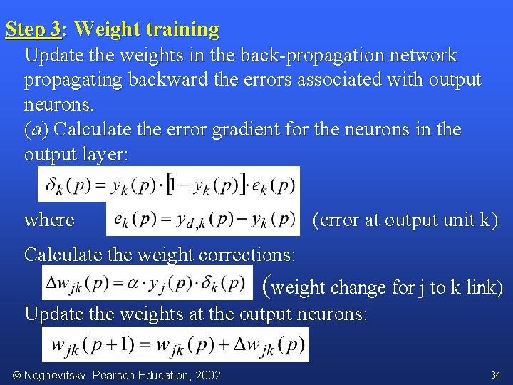
Step 3: Weight training Update the weights in the back-propagation network propagating backward the errors associated with output neurons. (a) Calculate the error gradient for the neurons in the output layer: where (error at output unit k) Calculate the weight corrections: (weight change for j to k link) Update the weights at the output neurons: Negnevitsky, Pearson Education, 2002 34

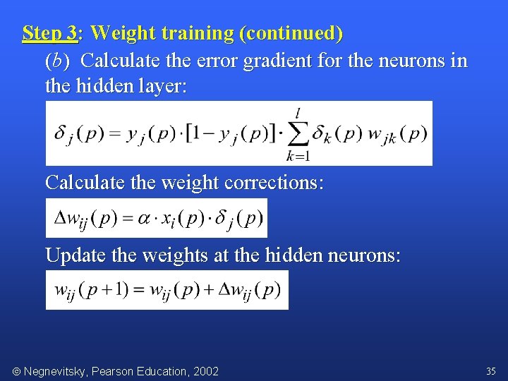
Step 3: Weight training (continued) (b) Calculate the error gradient for the neurons in the hidden layer: Calculate the weight corrections: Update the weights at the hidden neurons: Negnevitsky, Pearson Education, 2002 35

Step 4: Iteration Increase iteration p by one, go back to Step 2 and repeat the process until the selected error criterion is satisfied. Negnevitsky, Pearson Education, 2002 36

Example • network is required to perform logical operation Exclusive-OR. • Recall that a single-layer perceptron could not do this operation. • Now we will apply the three-layer backpropagation network • See Back. Prop. Learning. Xor. xls Negnevitsky, Pearson Education, 2002 37

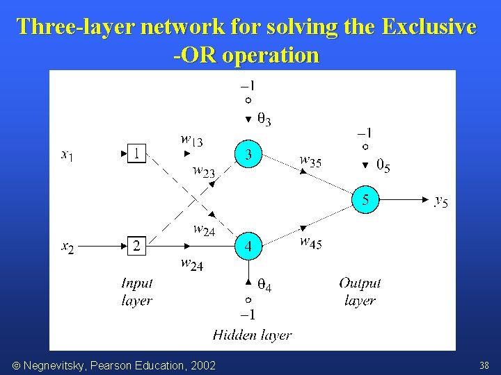
Three-layer network for solving the Exclusive -OR operation Negnevitsky, Pearson Education, 2002 38

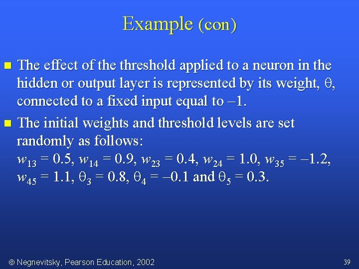
Example (con) The effect of the threshold applied to a neuron in the hidden or output layer is represented by its weight, , connected to a fixed input equal to 1. n The initial weights and threshold levels are set randomly as follows: w 13 = 0. 5, w 14 = 0. 9, w 23 = 0. 4, w 24 = 1. 0, w 35 = 1. 2, w 45 = 1. 1, 3 = 0. 8, 4 = 0. 1 and 5 = 0. 3. n Negnevitsky, Pearson Education, 2002 39

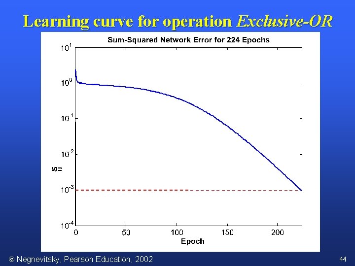
Learning curve for operation Exclusive-OR Negnevitsky, Pearson Education, 2002 44

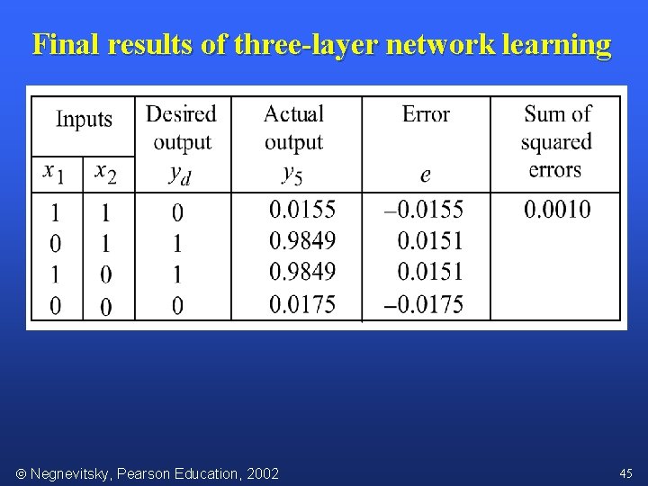
Final results of three-layer network learning Negnevitsky, Pearson Education, 2002 45

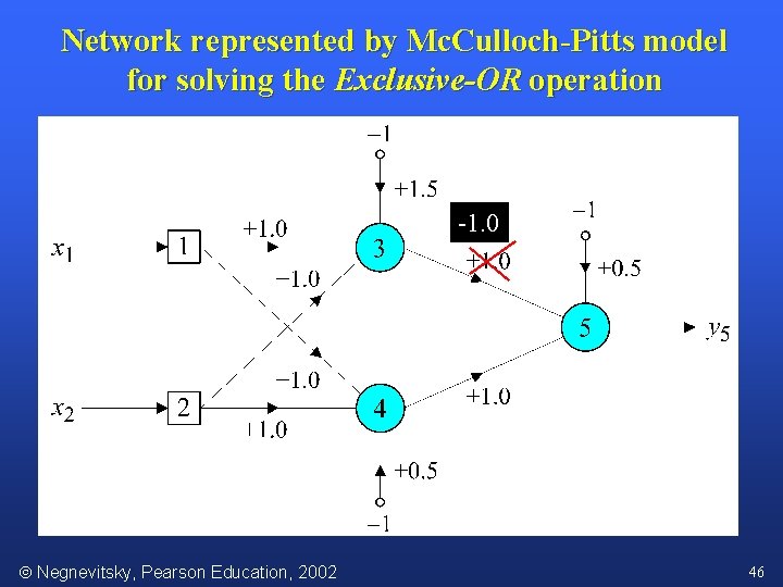
Network represented by Mc. Culloch-Pitts model for solving the Exclusive-OR operation -1. 0 Negnevitsky, Pearson Education, 2002 46

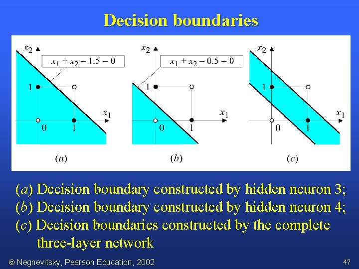
Decision boundaries (a) Decision boundary constructed by hidden neuron 3; (b) Decision boundary constructed by hidden neuron 4; (c) Decision boundaries constructed by the complete three-layer network Negnevitsky, Pearson Education, 2002 47

Neural Nets in Weka Xor – with default hidden layer n Xor – with two hidden nodes n Basketball Class n Broadway Stratified – default n Broadway Stratified – 10 hidden nodes n Negnevitsky, Pearson Education, 2002 48

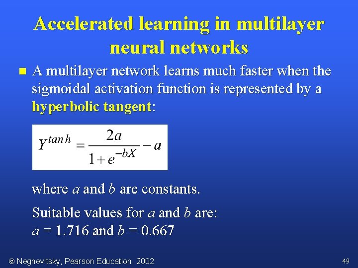
Accelerated learning in multilayer neural networks n A multilayer network learns much faster when the sigmoidal activation function is represented by a hyperbolic tangent: where a and b are constants. Suitable values for a and b are: a = 1. 716 and b = 0. 667 Negnevitsky, Pearson Education, 2002 49

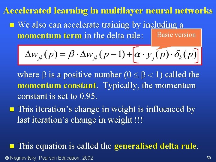
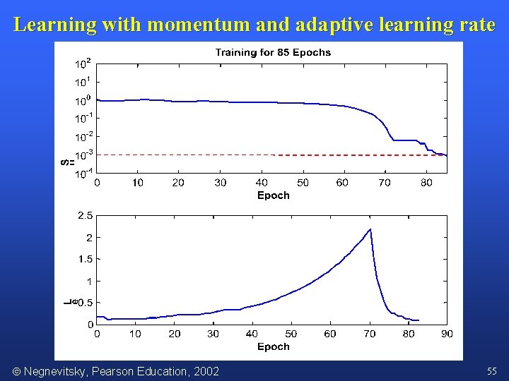
Accelerated learning in multilayer neural networks n We also can accelerate training by including a Basic version momentum term in the delta rule: where is a positive number (0 1) called the momentum constant. Typically, the momentum constant is set to 0. 95. n This iteration’s change in weight is influenced by last iteration’s change in weight !!! n This equation is called the generalised delta rule. Negnevitsky, Pearson Education, 2002 50

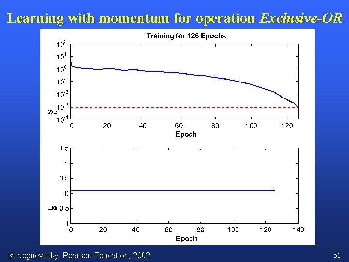
Learning with momentum for operation Exclusive-OR Negnevitsky, Pearson Education, 2002 51

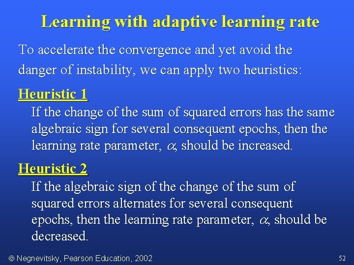
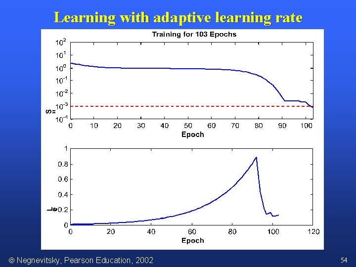
Learning with adaptive learning rate To accelerate the convergence and yet avoid the danger of instability, we can apply two heuristics: Heuristic 1 If the change of the sum of squared errors has the same algebraic sign for several consequent epochs, then the learning rate parameter, , should be increased. Heuristic 2 If the algebraic sign of the change of the sum of squared errors alternates for several consequent epochs, then the learning rate parameter, , should be decreased. Negnevitsky, Pearson Education, 2002 52

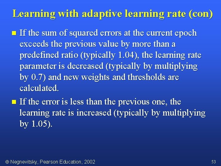
Learning with adaptive learning rate (con) If the sum of squared errors at the current epoch exceeds the previous value by more than a predefined ratio (typically 1. 04), the learning rate parameter is decreased (typically by multiplying by 0. 7) and new weights and thresholds are calculated. n If the error is less than the previous one, the learning rate is increased (typically by multiplying by 1. 05). n Negnevitsky, Pearson Education, 2002 53

Learning with adaptive learning rate Negnevitsky, Pearson Education, 2002 54

Learning with momentum and adaptive learning rate Negnevitsky, Pearson Education, 2002 55

End Neural Networks Negnevitsky, Pearson Education, 2002 56