Chapter 6 Analysis of Sequential Systems 5 1

Chapter 6 Analysis of Sequential Systems 5 1

Chapter 6 Analysis of Sequential Systems 6. 0 Introduction < Clocked System • Clock • A signal that alternates between 0 and 1 at a regular rate • Two versions of clock • Type A : 0 half and 1 half • Type B : 1 is shorter part of the cycle 5 P. 277 2

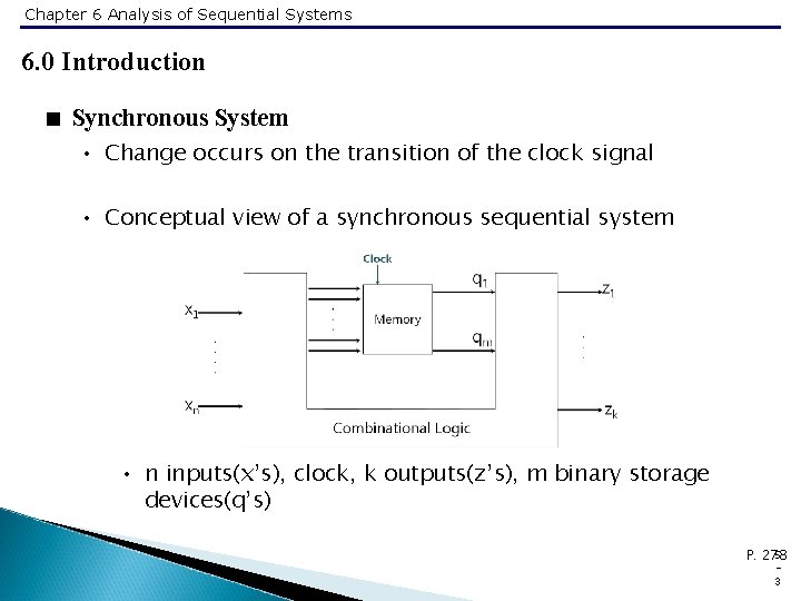
Chapter 6 Analysis of Sequential Systems 6. 0 Introduction < Synchronous System • Change occurs on the transition of the clock signal • Conceptual view of a synchronous sequential system • n inputs(x’s), clock, k outputs(z’s), m binary storage devices(q’s) 5 P. 278 3

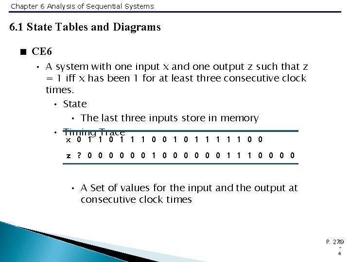
Chapter 6 Analysis of Sequential Systems 6. 1 State Tables and Diagrams < CE 6 • A system with one input x and one output z such that z = 1 iff x has been 1 for at least three consecutive clock times. • State • The last three inputs store in memory • Timing Trace x 0 1 1 1 0 0 z ? 0 0 0 1 1 1 0 0 • A Set of values for the input and the output at consecutive clock times 5 P. 279 4

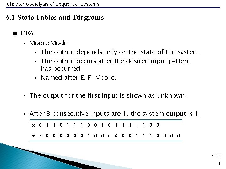
Chapter 6 Analysis of Sequential Systems 6. 1 State Tables and Diagrams < CE 6 • Moore Model • The output depends only on the state of the system. • The output occurs after the desired input pattern has occurred. • Named after E. F. Moore. • The output for the first input is shown as unknown. • After 3 consecutive inputs are 1, the system output is 1. x 0 1 1 1 0 0 z ? 0 0 0 1 1 1 0 0 5 P. 278 5

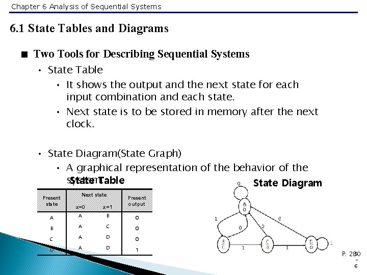
Chapter 6 Analysis of Sequential Systems 6. 1 State Tables and Diagrams < Two Tools for Describing Sequential Systems • State Table • It shows the output and the next state for each input combination and each state. • Next state is to be stored in memory after the next clock. • State Diagram(State Graph) • A graphical representation of the behavior of the system. State Table State Diagram Present state Next state Present output x=0 x=1 A A B 0 B A C 0 C A D 0 D A D 1 5 P. 280 6

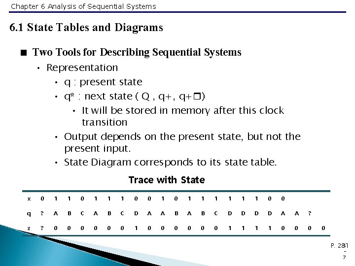
Chapter 6 Analysis of Sequential Systems 6. 1 State Tables and Diagrams < Two Tools for Describing Sequential Systems • Representation • q : present state • q* : next state ( Q , q+ ) • It will be stored in memory after this clock transition • Output depends on the present state, but not the present input. • State Diagram corresponds to its state table. Trace with State x 0 1 1 1 0 0 1 1 1 1 0 0 q ? A B C D A A B C D D A A ? z ? 0 0 0 1 1 1 1 0 0 5 P. 281 7

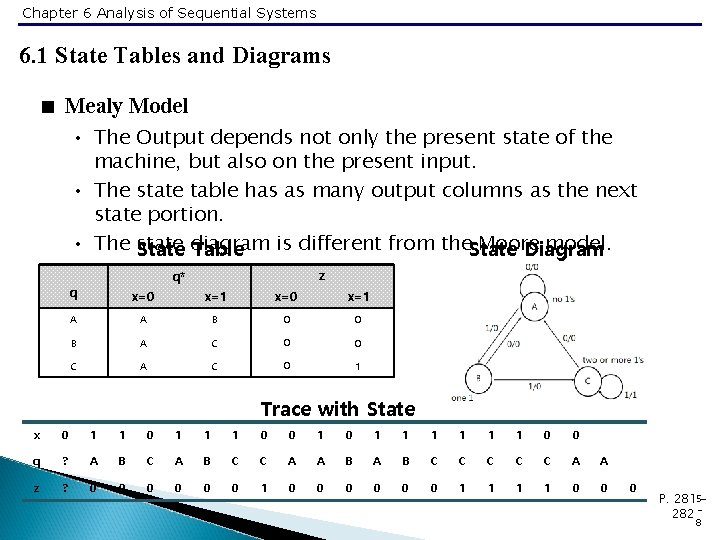
Chapter 6 Analysis of Sequential Systems 6. 1 State Tables and Diagrams < Mealy Model • The Output depends not only the present state of the machine, but also on the present input. • The state table has as many output columns as the next state portion. • The state is different from the. State Moore model. State diagram Table Diagram z q* q x=0 x=1 A A B 0 0 B A C 0 0 C A C 0 1 Trace with State x 0 1 1 1 0 0 1 1 1 1 0 0 q ? A B C C A A B C C C A A z ? 0 0 0 1 1 1 1 0 0 0 P. 2815282 8

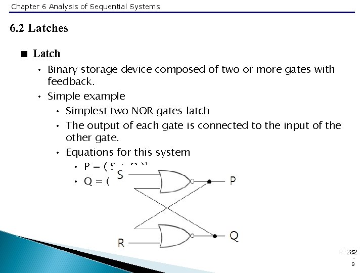
Chapter 6 Analysis of Sequential Systems 6. 2 Latches < Latch • Binary storage device composed of two or more gates with feedback. • Simple example • Simplest two NOR gates latch • The output of each gate is connected to the input of the other gate. • Equations for this system • P = ( S + Q )’ • Q = ( R + P )’ 5 P. 282 9

Chapter 6 Analysis of Sequential Systems 6. 2 Latches < Latch • Simple example • Equations for this system • S = 0, R = 0 • P = Q’, Q = P’ • Store 0 (Q = 0 and P = 1) or store 1 (Q = 1 and P = 0) • S is used to indicate ‘set’, store a 1 in the latch • S=1, R=0 • P = (1 + Q)’ = 1’ = 0 • Q = (0 + 0)’ = 0’ = 1 • R is used to indicate ‘reset’, store a 0 in the latch • S=0, R=1 • Q = (1 + P)’ = 1’ = 0 • P = (0 + 0)’ = 0’ = 1 5 10

Chapter 6 Analysis of Sequential Systems 6. 2 Latches < Latch • Simple example • Equations for this system • S = 1 , R = 1 : not operated • P = (1 + Q)’ = 1’ = 0 • Q = (1 + P)’ = 1’ = 0 5 11

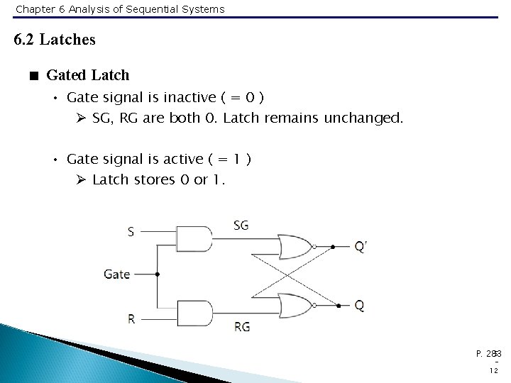
Chapter 6 Analysis of Sequential Systems 6. 2 Latches < Gated Latch • Gate signal is inactive ( = 0 ) Ø SG, RG are both 0. Latch remains unchanged. • Gate signal is active ( = 1 ) Ø Latch stores 0 or 1. 5 P. 283 12

Chapter 6 Analysis of Sequential Systems 6. 3 Flip Flops < Flip Flop • Clocked binary storage device • Flip Flop stores a 0 or a 1. • Trailing-edge Triggered • Change FF state when the clock goes from 1 to 0. • Leading-edge Triggered • Change FF state when the clock goes from 0 to 1. • Various Types of Flip Flops • D Flip Flop • JK Flip Flop • SR Flip Flop • T Flip Flop 5 13

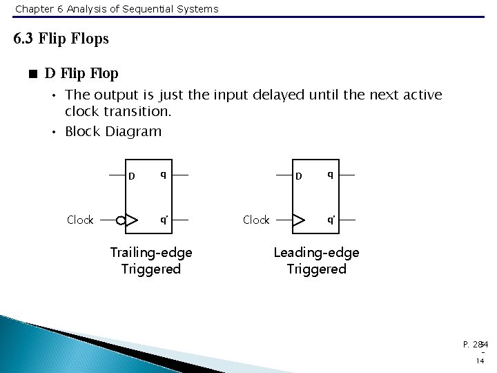
Chapter 6 Analysis of Sequential Systems 6. 3 Flip Flops < D Flip Flop • The output is just the input delayed until the next active clock transition. • Block Diagram D Clock q q’ Trailing-edge Triggered D Clock q q’ Leading-edge Triggered 5 P. 284 14

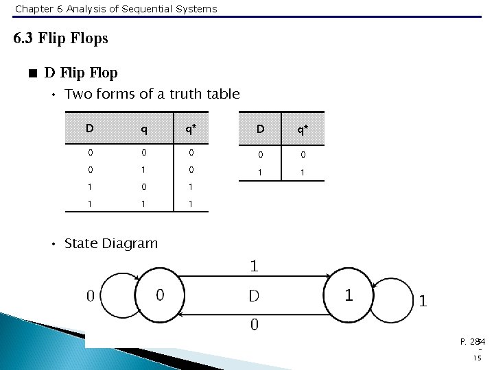
Chapter 6 Analysis of Sequential Systems 6. 3 Flip Flops < D Flip Flop • Two forms of a truth table D q q* D q* 0 0 0 1 0 1 1 1 1 • State Diagram 5 P. 284 15

Chapter 6 Analysis of Sequential Systems 6. 3 Flip Flops < D Flip Flop • Timing Diagram • Trailing-edge triggered D FF • Result in (b) will be same as (a) (b) 5 P. 285 16

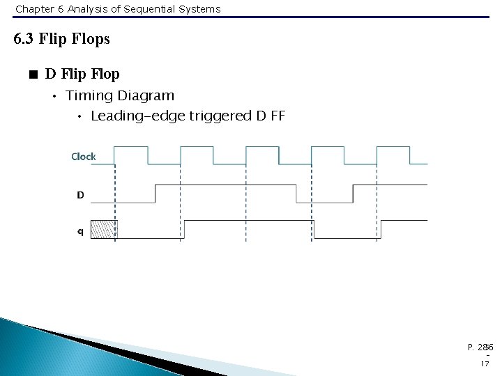
Chapter 6 Analysis of Sequential Systems 6. 3 Flip Flops < D Flip Flop • Timing Diagram • Leading-edge triggered D FF 5 P. 286 17

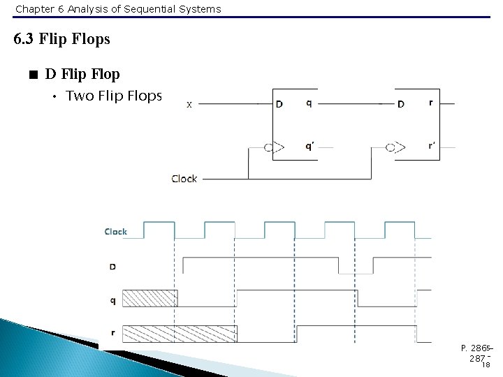
Chapter 6 Analysis of Sequential Systems 6. 3 Flip Flops < D Flip Flop • Two Flip Flops P. 2865287 18

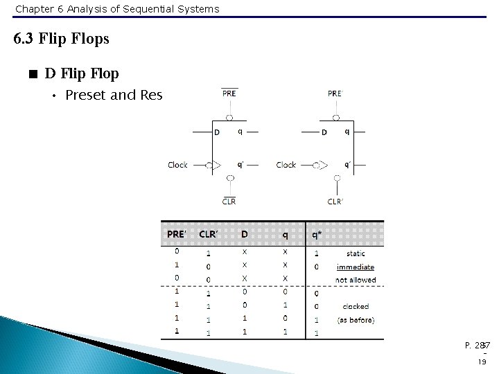
Chapter 6 Analysis of Sequential Systems 6. 3 Flip Flops < D Flip Flop • Preset and Reset 5 P. 287 19

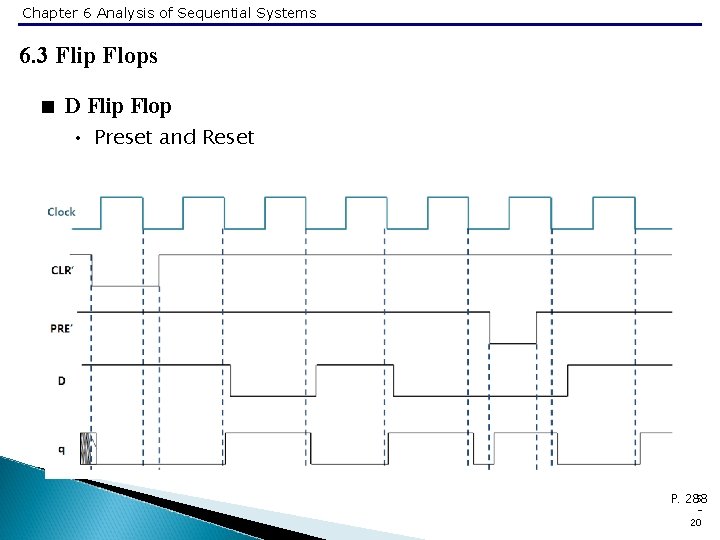
Chapter 6 Analysis of Sequential Systems 6. 3 Flip Flops < D Flip Flop • Preset and Reset 5 P. 288 20

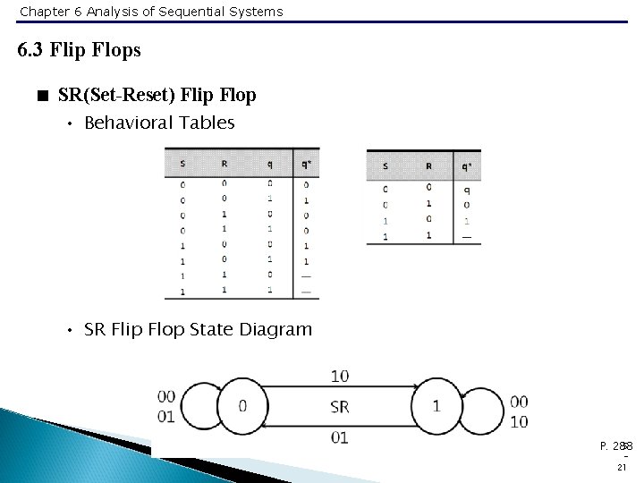
Chapter 6 Analysis of Sequential Systems 6. 3 Flip Flops < SR(Set-Reset) Flip Flop • Behavioral Tables • SR Flip Flop State Diagram 5 P. 288 21

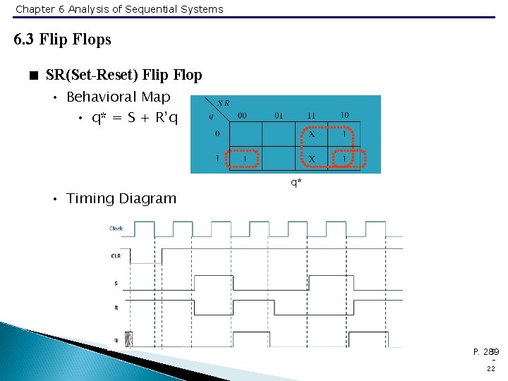
Chapter 6 Analysis of Sequential Systems 6. 3 Flip Flops < SR(Set-Reset) Flip Flop • Behavioral Map • q* = S + R’q • Timing Diagram q* 5 P. 289 22

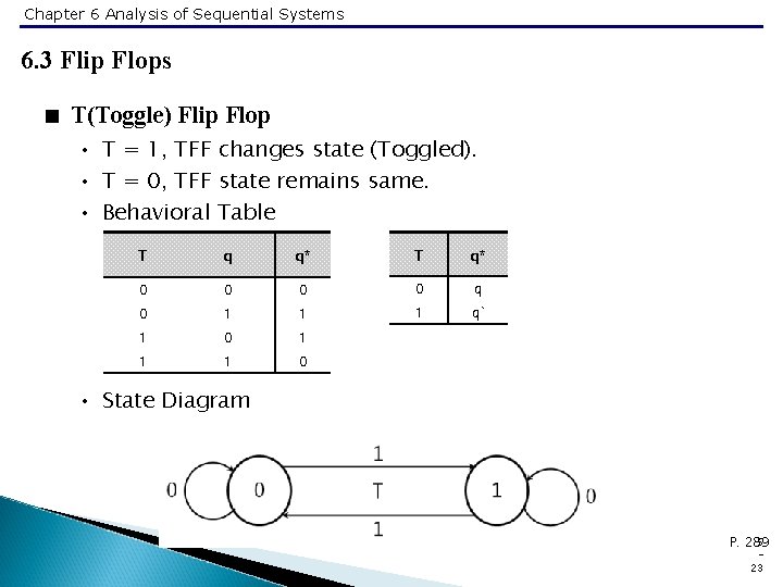
Chapter 6 Analysis of Sequential Systems 6. 3 Flip Flops < T(Toggle) Flip Flop • T = 1, TFF changes state (Toggled). • T = 0, TFF state remains same. • Behavioral Table T q q* T q* 0 0 q 0 1 1 1 q` 1 0 1 1 1 0 • State Diagram 5 P. 289 23

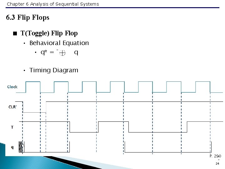
Chapter 6 Analysis of Sequential Systems 6. 3 Flip Flops < T(Toggle) Flip Flop • Behavioral Equation • q* = T q • Timing Diagram 5 P. 290 24

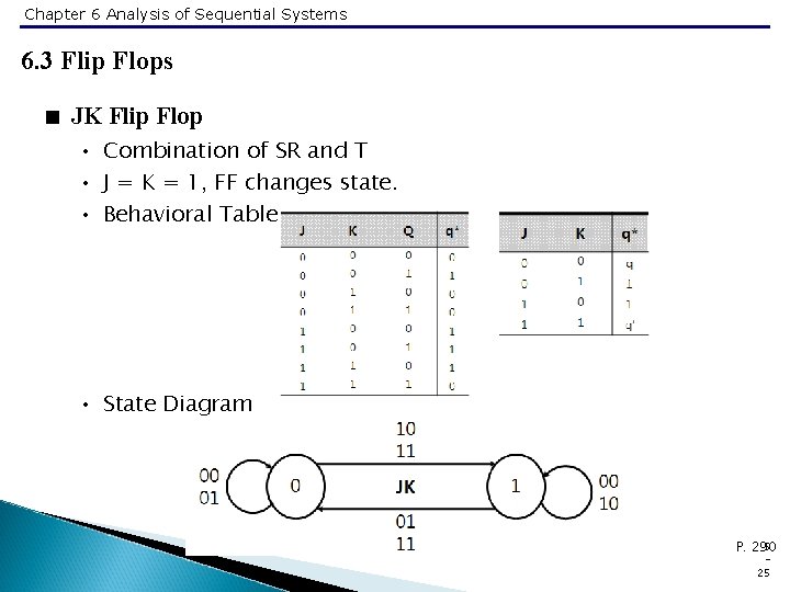
Chapter 6 Analysis of Sequential Systems 6. 3 Flip Flops < JK Flip Flop • Combination of SR and T • J = K = 1, FF changes state. • Behavioral Table • State Diagram 5 P. 290 25

Chapter 6 Analysis of Sequential Systems 6. 3 Flip Flops < JK Flip Flop • Behavioral Equation • q* = Jq’ + K’q • Timing Diagram 5 P. 291 26

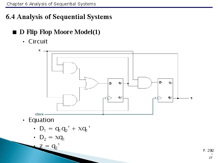
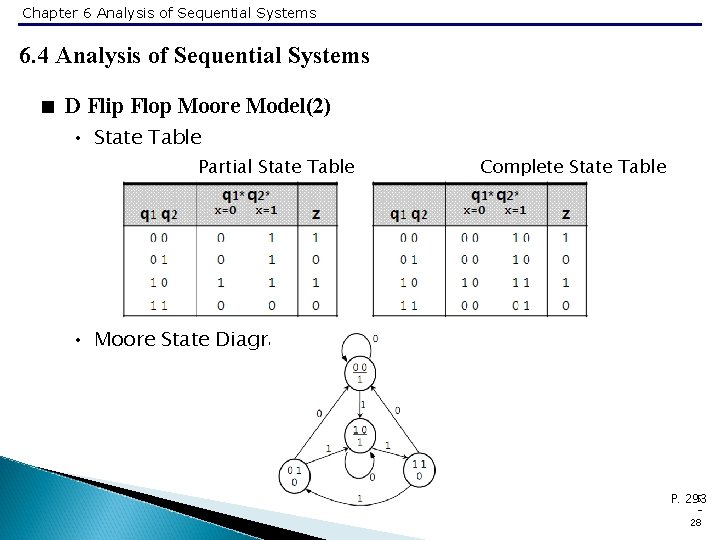
Chapter 6 Analysis of Sequential Systems 6. 4 Analysis of Sequential Systems < D Flip Flop Moore Model(1) • Circuit • Equation • D 1 = q 1 q 2’ + xq 1’ • D 2 = xq 1 • z = q 2’ 5 P. 292 27

Chapter 6 Analysis of Sequential Systems 6. 4 Analysis of Sequential Systems < D Flip Flop Moore Model(2) • State Table Partial State Table Complete State Table • Moore State Diagram 5 P. 293 28

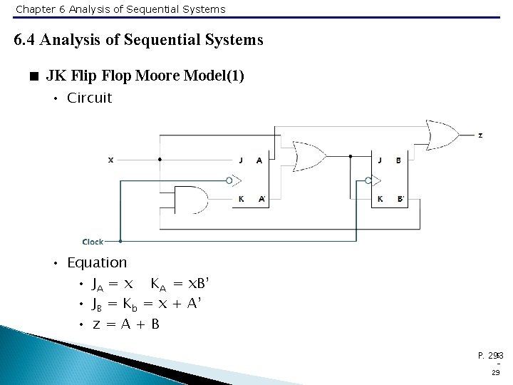
Chapter 6 Analysis of Sequential Systems 6. 4 Analysis of Sequential Systems < JK Flip Flop Moore Model(1) • Circuit • Equation • JA = x KA = x. B’ • JB = Kb = x + A’ • z=A+B 5 P. 293 29

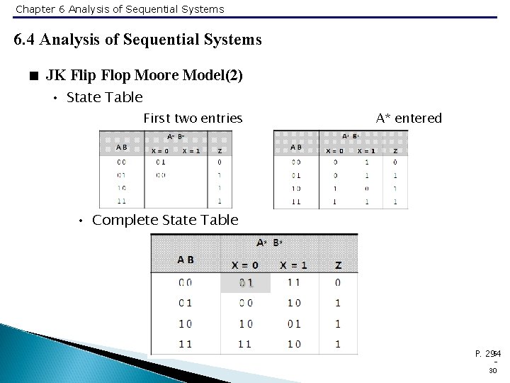
Chapter 6 Analysis of Sequential Systems 6. 4 Analysis of Sequential Systems < JK Flip Flop Moore Model(2) • State Table First two entries A* entered • Complete State Table 5 P. 294 30

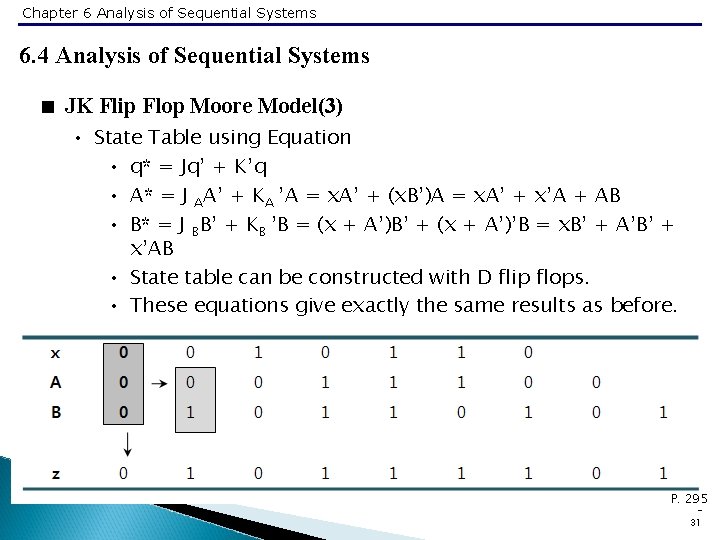
Chapter 6 Analysis of Sequential Systems 6. 4 Analysis of Sequential Systems < JK Flip Flop Moore Model(3) • State Table using Equation • q* = Jq’ + K’q • A* = J AA’ + KA ’A = x. A’ + (x. B’)A = x. A’ + x’A + AB • B* = J BB’ + KB ’B = (x + A’)B’ + (x + A’)’B = x. B’ + A’B’ + x’AB • State table can be constructed with D flip flops. • These equations give exactly the same results as before. • Trace Table 5 P. 295 31

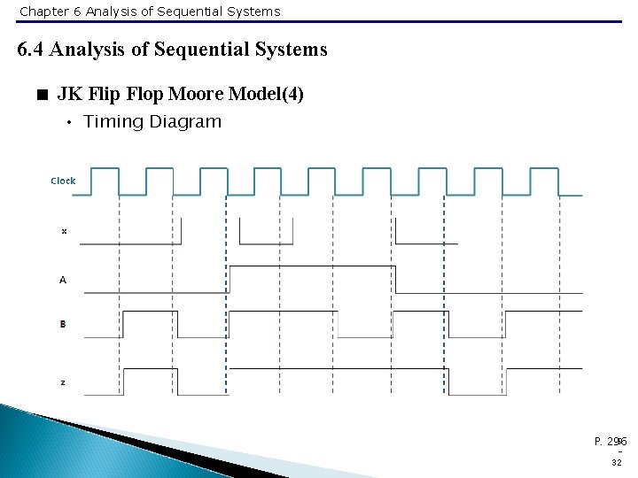
Chapter 6 Analysis of Sequential Systems 6. 4 Analysis of Sequential Systems < JK Flip Flop Moore Model(4) • Timing Diagram 5 P. 296 32

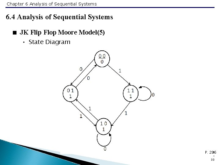
Chapter 6 Analysis of Sequential Systems 6. 4 Analysis of Sequential Systems < JK Flip Flop Moore Model(5) • State Diagram 5 P. 296 33

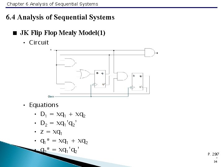
Chapter 6 Analysis of Sequential Systems 6. 4 Analysis of Sequential Systems < JK Flip Flop Mealy Model(1) • Circuit • Equations • D 1 = xq 1 + xq 2 • D 2 = xq 1’q 2’ • z = xq 1 • q 1* = xq 1 + xq 2 • q 2* = xq 1’q 2’ 5 P. 297 34

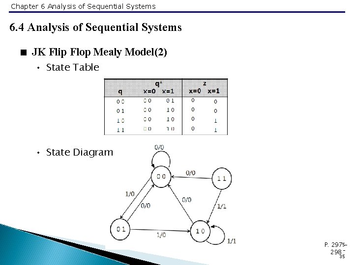
Chapter 6 Analysis of Sequential Systems 6. 4 Analysis of Sequential Systems < JK Flip Flop Mealy Model(2) • State Table • State Diagram P. 2975298 35

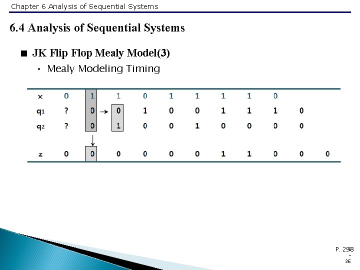
Chapter 6 Analysis of Sequential Systems 6. 4 Analysis of Sequential Systems < JK Flip Flop Mealy Model(3) • Mealy Modeling Timing 5 P. 298 36

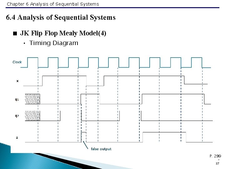
Chapter 6 Analysis of Sequential Systems 6. 4 Analysis of Sequential Systems < JK Flip Flop Mealy Model(4) • Timing Diagram 5 P. 299 37

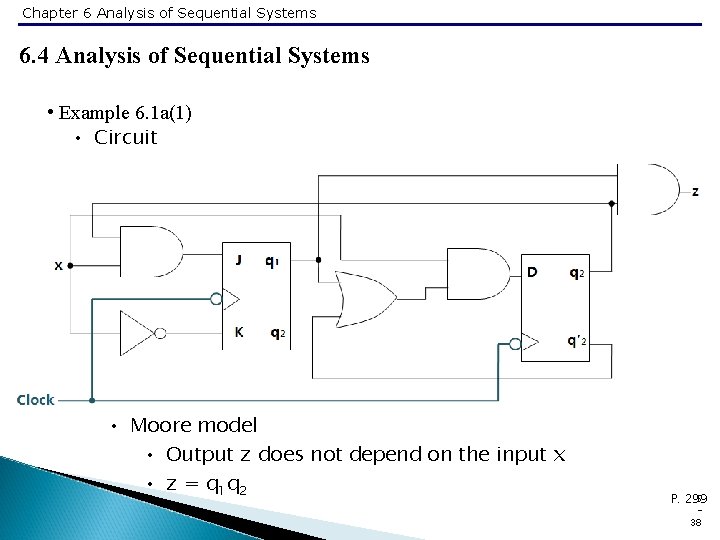
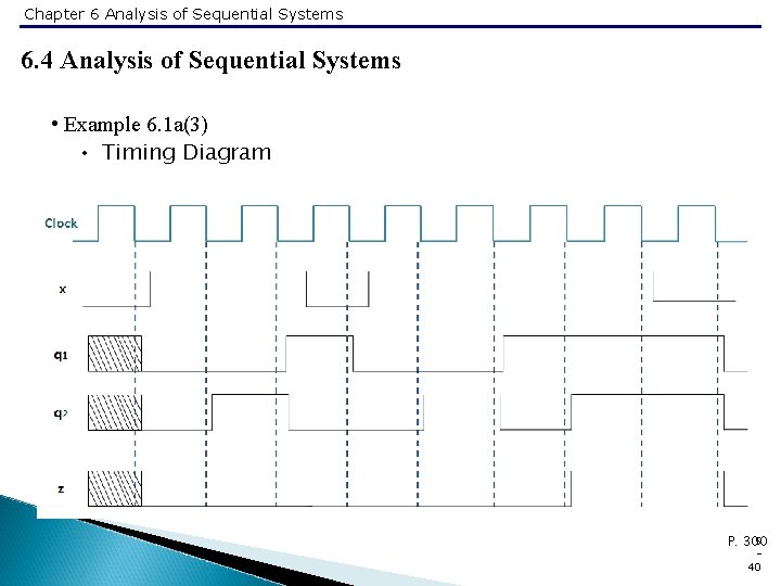
Chapter 6 Analysis of Sequential Systems 6. 4 Analysis of Sequential Systems • Example 6. 1 a(1) • Circuit • Moore model • Output z does not depend on the input x • z = q 1 q 2 5 P. 299 38

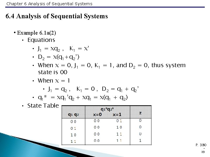
Chapter 6 Analysis of Sequential Systems 6. 4 Analysis of Sequential Systems • Example 6. 1 a(2) • Equations • J 1 = xq 2 , K 1 = x’ • D 2 = x(q 1+q 2’) • When x = 0, J 1 = 0, K 1 = 1, and D 2 = 0, thus system state is 00 • When x = 1 • J 1 = q 2 , K 1 = 0 , D 2 = q 1 + q 2 ’ • q 1* = xq 1’q 2 + xq 1 = x(q 1 + q 2) • State Table 5 P. 300 39

Chapter 6 Analysis of Sequential Systems 6. 4 Analysis of Sequential Systems • Example 6. 1 a(3) • Timing Diagram 5 P. 300 40

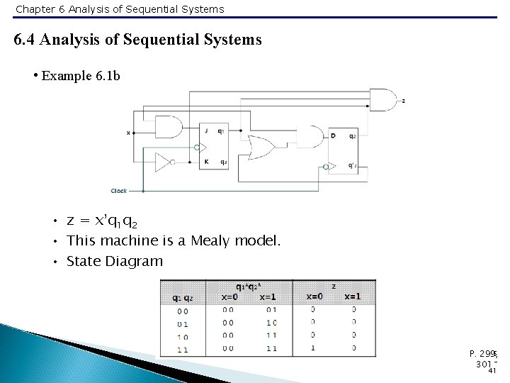
Chapter 6 Analysis of Sequential Systems 6. 4 Analysis of Sequential Systems • Example 6. 1 b • z = x’q 1 q 2 • This machine is a Mealy model. • State Diagram 5 P. 299, 301 41

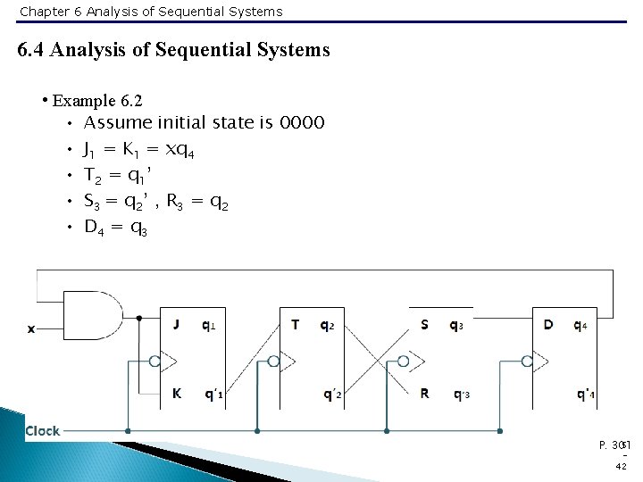
Chapter 6 Analysis of Sequential Systems 6. 4 Analysis of Sequential Systems • Example 6. 2 • Assume initial state is 0000 • J 1 = K 1 = xq 4 • T 2 = q 1 ’ • S 3 = q 2 ’ , R 3 = q 2 • D 4 = q 3 5 P. 301 42

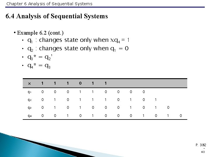
Chapter 6 Analysis of Sequential Systems 6. 4 Analysis of Sequential Systems • Example 6. 2 (cont. ) • q 1 : changes state only when xq 4 = 1 • q 2 : changes state only when q 1 = 0 • q 3 * = q 2 ’ • q 4 * = q 3 x 1 1 1 0 1 1 q 1 0 0 0 1 1 0 0 q 2 0 1 1 1 0 1 q 3 0 1 0 0 0 1 0 q 4 0 0 1 0 1 0 5 P. 302 43