Chapter 53 Population Ecology Power Point Lecture Presentations

Chapter 53 Population Ecology Power. Point® Lecture Presentations for Biology Eighth Edition Neil Campbell and Jane Reece Lectures by Chris Romero, updated by Erin Barley with contributions from Joan Sharp Copyright © 2008 Pearson Education, Inc. , publishing as Pearson Benjamin Cummings

Overview • Population ecology is the study of populations in relation to environment, including environmental influences on density and distribution, age structure, and population size. • A population is a group of individuals of a single species living in the same general area. Copyright © 2008 Pearson Education, Inc. , publishing as Pearson Benjamin Cummings

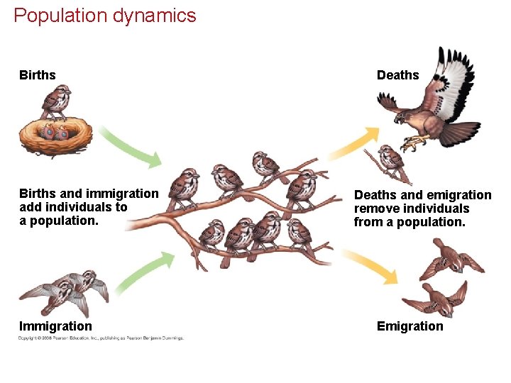
Dynamic biological processes influence population density, dispersion, and demographics • Density is the number of individuals per unit area or volume. • Dispersion is the pattern of spacing among individuals within the boundaries of the population. • Density is the result of an interplay between processes that add individuals to a population and those that remove individuals. Copyright © 2008 Pearson Education, Inc. , publishing as Pearson Benjamin Cummings

• Immigration is the influx of new individuals from other areas. • Emigration is the movement of individuals out of a population. • In most cases, it is impractical or impossible to count all individuals in a population. Sampling techniques can be used to estimate densities and total population sizes. • Population size can be estimated by either extrapolation from small samples, an index of population size, or the Mark-Recapture Method. Copyright © 2008 Pearson Education, Inc. , publishing as Pearson Benjamin Cummings

Population dynamics Births and immigration add individuals to a population. Immigration Deaths and emigration remove individuals from a population. Emigration

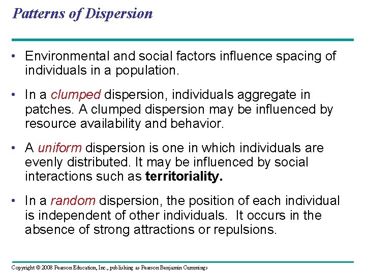
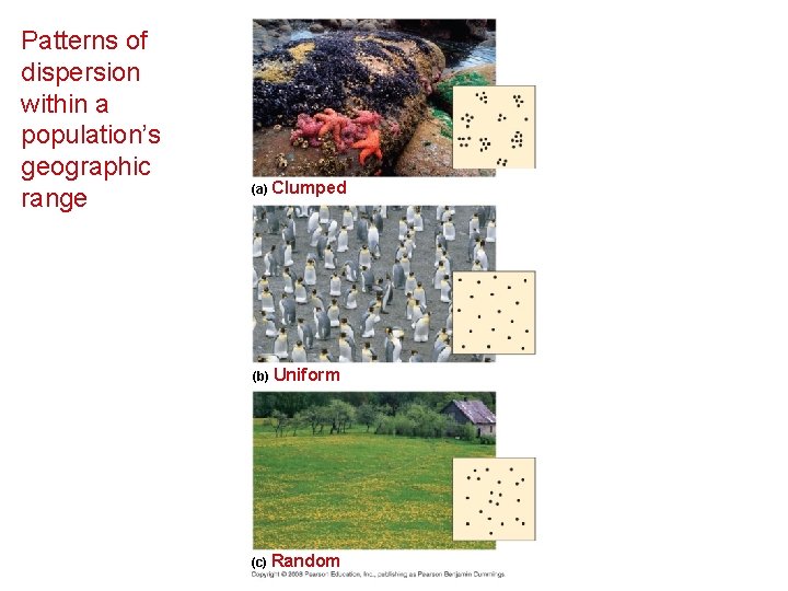
Patterns of Dispersion • Environmental and social factors influence spacing of individuals in a population. • In a clumped dispersion, individuals aggregate in patches. A clumped dispersion may be influenced by resource availability and behavior. • A uniform dispersion is one in which individuals are evenly distributed. It may be influenced by social interactions such as territoriality. • In a random dispersion, the position of each individual is independent of other individuals. It occurs in the absence of strong attractions or repulsions. Copyright © 2008 Pearson Education, Inc. , publishing as Pearson Benjamin Cummings

Patterns of dispersion within a population’s geographic range (a) Clumped (b) Uniform (c) Random

Demographics • Demography is the study of the vital statistics of a population and how they change over time. • Death rates and birth rates are of particular interest to demographers. Copyright © 2008 Pearson Education, Inc. , publishing as Pearson Benjamin Cummings

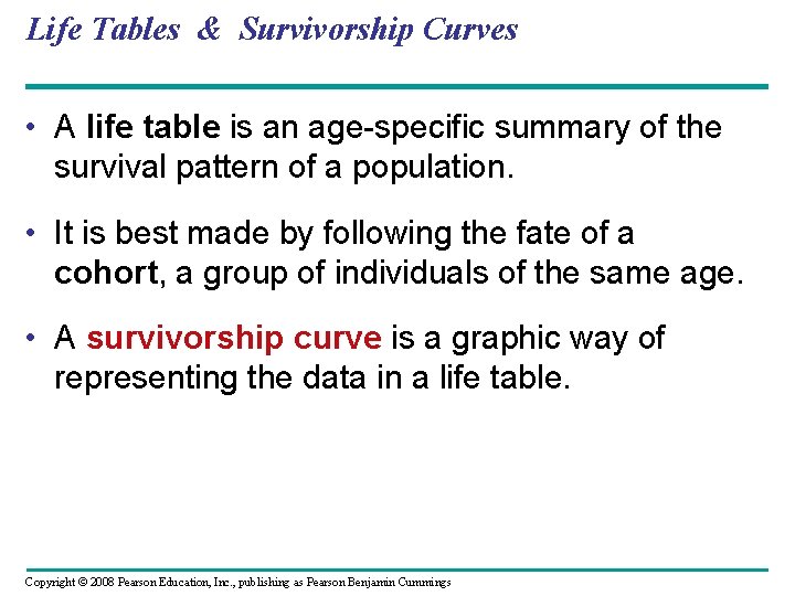
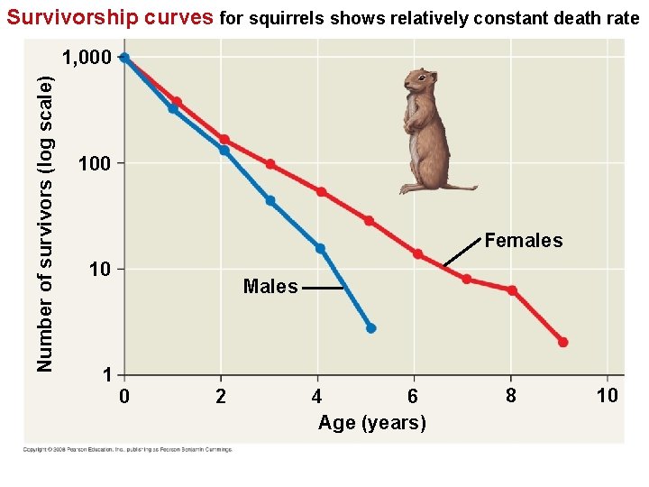
Life Tables & Survivorship Curves • A life table is an age-specific summary of the survival pattern of a population. • It is best made by following the fate of a cohort, a group of individuals of the same age. • A survivorship curve is a graphic way of representing the data in a life table. Copyright © 2008 Pearson Education, Inc. , publishing as Pearson Benjamin Cummings

Survivorship curves for squirrels shows relatively constant death rate Number of survivors (log scale) 1, 000 100 Females 10 1 Males 0 2 4 6 Age (years) 8 10

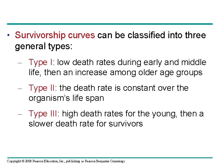
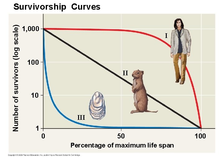
• Survivorship curves can be classified into three general types: – Type I: low death rates during early and middle life, then an increase among older age groups – Type II: the death rate is constant over the organism’s life span – Type III: high death rates for the young, then a slower death rate for survivors Copyright © 2008 Pearson Education, Inc. , publishing as Pearson Benjamin Cummings

Number of survivors (log scale) Survivorship Curves 1, 000 I 100 II 10 III 1 0 50 Percentage of maximum life span 100

Reproductive Rates • For species with sexual reproduction, demographers often concentrate on females in a population. • A reproductive table, or fertility schedule, is an age-specific summary of the reproductive rates in a population. It describes reproductive patterns of a population. Copyright © 2008 Pearson Education, Inc. , publishing as Pearson Benjamin Cummings

Life history traits are products of natural selection • An organism’s life history comprises the traits that affect its schedule of reproduction and survival: – The age at which reproduction begins – How often the organism reproduces – How many offspring are produced during each reproductive cycle • Life history traits are evolutionary outcomes reflected in the development, physiology, and behavior of an organism. Copyright © 2008 Pearson Education, Inc. , publishing as Pearson Benjamin Cummings

Evolution and Life History Diversity • Life histories are very diverse. • Species that exhibit semelparity, or big-bang reproduction, reproduce once and die. • Species that exhibit iteroparity, or repeated reproduction, produce offspring repeatedly. • Highly variable or unpredictable environments likely favor big-bang reproduction, while dependable environments may favor repeated reproduction. Copyright © 2008 Pearson Education, Inc. , publishing as Pearson Benjamin Cummings

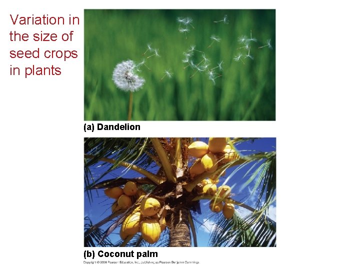
“Trade-offs” and Life Histories • Organisms have finite resources, which may lead to trade-offs between survival and reproduction. • In animals, parental care of smaller broods may facilitate survival of offspring. • Some plants, like the dandelion, produce a large number of small seeds, ensuring that at least some of them will grow and eventually reproduce. • Other types of plants, like the coconut tree, produce a moderate number of large seeds that provide a large store of energy that will help seedlings become established. Copyright © 2008 Pearson Education, Inc. , publishing as Pearson Benjamin Cummings

Variation in the size of seed crops in plants (a) Dandelion (b) Coconut palm

The exponential model describes population growth in an idealized, unlimited environment • It is useful to study population growth in an idealized situation. • Idealized situations help us understand the capacity of species to increase and the conditions that may facilitate this growth. Copyright © 2008 Pearson Education, Inc. , publishing as Pearson Benjamin Cummings

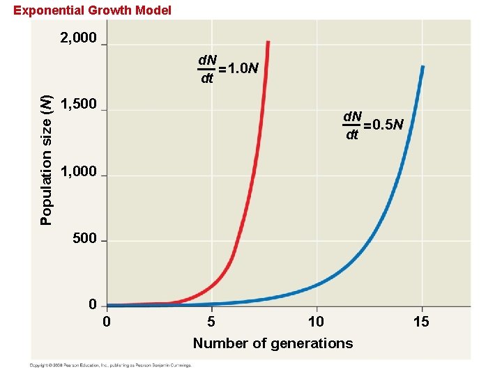
• Zero population growth occurs when the birth rate equals the death rate. • Most ecologists use differential calculus to express population growth as growth rate at a particular instant in time: N r. N t where N = population size, t = time, and r = per capita rate of increase = birth – death Copyright © 2008 Pearson Education, Inc. , publishing as Pearson Benjamin Cummings

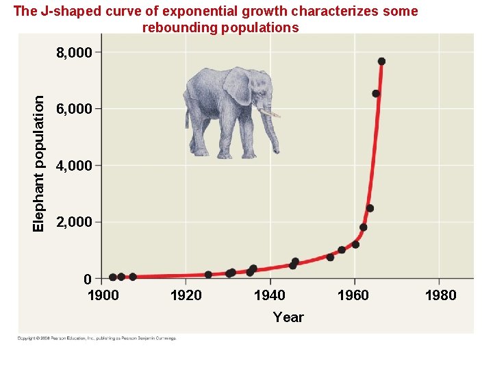
Exponential Growth • Exponential population growth is population increase under idealized conditions. • Under these conditions, the rate of reproduction is at its maximum, called the intrinsic rate of increase. • Exponential population growth results in a Jshaped curve • Exponential Growth is not sustainable. Copyright © 2008 Pearson Education, Inc. , publishing as Pearson Benjamin Cummings

Exponential Growth Model 2, 000 Population size (N) d. N = 1. 0 N dt 1, 500 d. N = 0. 5 N dt 1, 000 500 0 0 5 10 Number of generations 15

The J-shaped curve of exponential growth characterizes some rebounding populations Elephant population 8, 000 6, 000 4, 000 2, 000 0 1900 1920 1940 Year 1960 1980

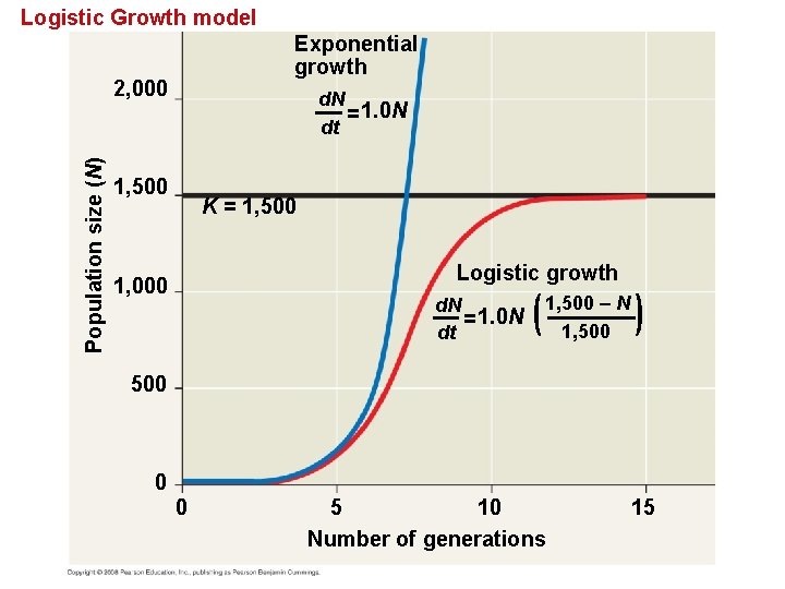
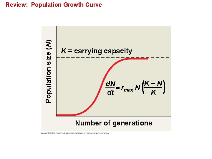
The logistic model describes how a population grows more slowly as it nears its carrying capacity • Exponential growth cannot be sustained for long in any population. A more realistic population model limits growth by incorporating carrying capacity. • Carrying capacity (K) is the maximum population size the environment can support. • In the logistic population growth model, the rate of increase declines as carrying capacity is reached. • The logistic model of population growth produces a sigmoid (S-shaped) curve. Copyright © 2008 Pearson Education, Inc. , publishing as Pearson Benjamin Cummings

Logistic Growth model Exponential growth Population size (N) 2, 000 d. N = 1. 0 N dt 1, 500 K = 1, 500 Logistic growth 1, 000 d. N = 1. 0 N dt 1, 500 – N 1, 500 0 0 5 10 Number of generations 15

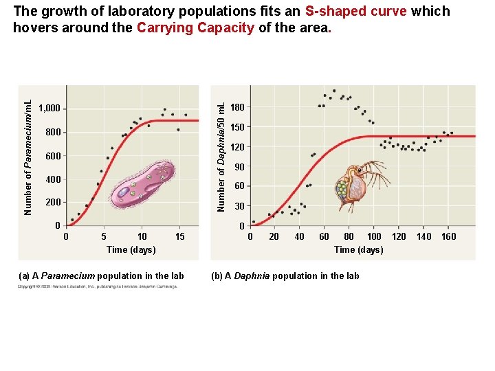
The Logistic Model and Real Populations • The growth of laboratory populations of paramecia fits an S-shaped curve. • These organisms are grown in a constant environment lacking predators and competitors. • Some populations overshoot K before settling down to a relatively stable density. Copyright © 2008 Pearson Education, Inc. , publishing as Pearson Benjamin Cummings

Number of Daphnia/50 m. L Number of Paramecium/m. L The growth of laboratory populations fits an S-shaped curve which hovers around the Carrying Capacity of the area. 1, 000 800 600 400 200 0 180 150 120 90 60 30 0 0 5 10 Time (days) 15 (a) A Paramecium population in the lab 0 20 40 60 80 100 120 Time (days) (b) A Daphnia population in the lab 140 160

The Logistic Model and Life Histories • Life history traits favored by natural selection may vary with population density and environmental conditions. • K-selection = density-dependent selection, selects for life history traits that are sensitive to population density. • r-selection = or density-independent selection, selects for life history traits that maximize reproduction. Copyright © 2008 Pearson Education, Inc. , publishing as Pearson Benjamin Cummings

Many factors that regulate population growth are density dependent • There are two general questions about regulation of population growth: – What environmental factors stop a population from growing indefinitely? – Why do some populations show radical fluctuations in size over time, while others remain stable? Copyright © 2008 Pearson Education, Inc. , publishing as Pearson Benjamin Cummings

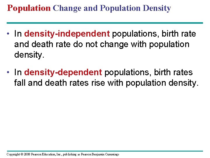
Population Change and Population Density • In density-independent populations, birth rate and death rate do not change with population density. • In density-dependent populations, birth rates fall and death rates rise with population density. Copyright © 2008 Pearson Education, Inc. , publishing as Pearson Benjamin Cummings

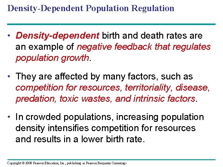
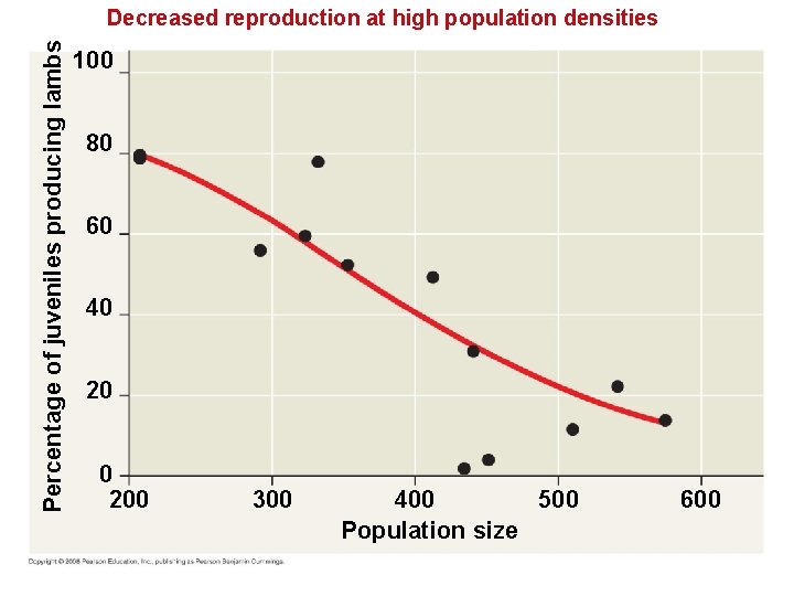
Density-Dependent Population Regulation • Density-dependent birth and death rates are an example of negative feedback that regulates population growth. • They are affected by many factors, such as competition for resources, territoriality, disease, predation, toxic wastes, and intrinsic factors. • In crowded populations, increasing population density intensifies competition for resources and results in a lower birth rate. Copyright © 2008 Pearson Education, Inc. , publishing as Pearson Benjamin Cummings

Percentage of juveniles producing lambs Decreased reproduction at high population densities 100 80 60 40 200 300 400 500 Population size 600

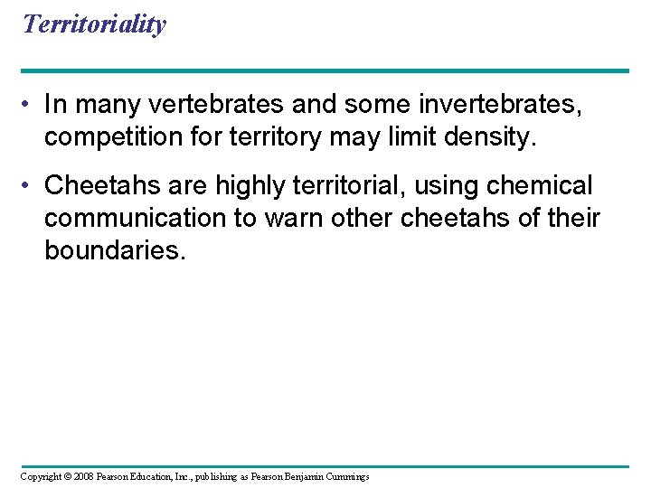
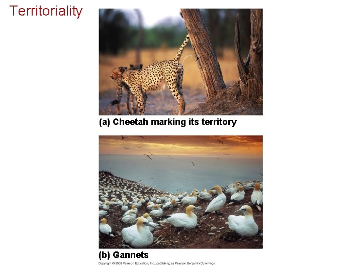
Territoriality • In many vertebrates and some invertebrates, competition for territory may limit density. • Cheetahs are highly territorial, using chemical communication to warn other cheetahs of their boundaries. Copyright © 2008 Pearson Education, Inc. , publishing as Pearson Benjamin Cummings

Territoriality (a) Cheetah marking its territory (b) Gannets

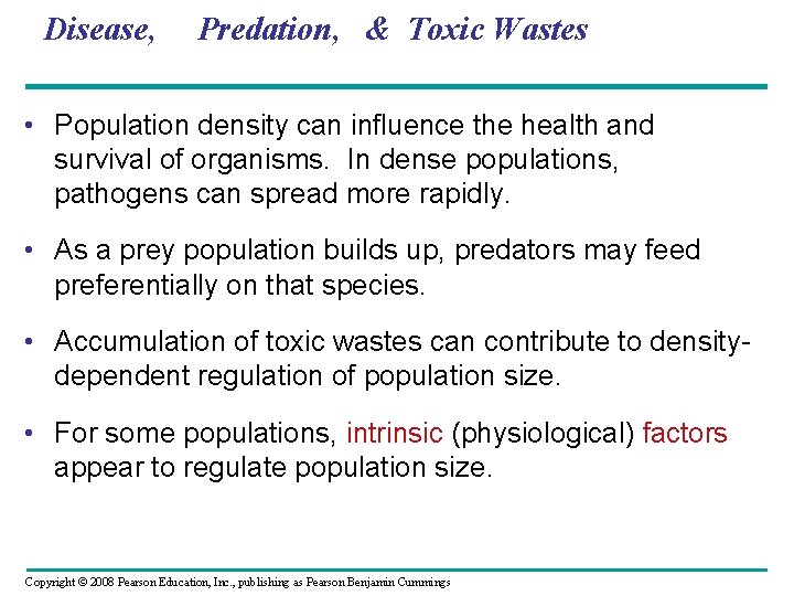
Disease, Predation, & Toxic Wastes • Population density can influence the health and survival of organisms. In dense populations, pathogens can spread more rapidly. • As a prey population builds up, predators may feed preferentially on that species. • Accumulation of toxic wastes can contribute to densitydependent regulation of population size. • For some populations, intrinsic (physiological) factors appear to regulate population size. Copyright © 2008 Pearson Education, Inc. , publishing as Pearson Benjamin Cummings

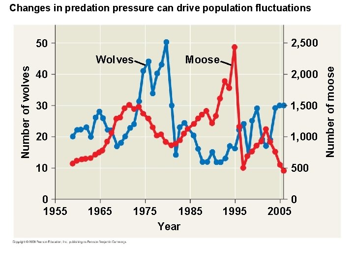
Population Dynamics • The study of population dynamics focuses on the complex interactions between biotic and abiotic factors that cause variation in population size. • Long-term population studies have challenged the hypothesis that populations of large mammals are relatively stable over time. • Weather can affect population size over time. Copyright © 2008 Pearson Education, Inc. , publishing as Pearson Benjamin Cummings

Changes in predation pressure can drive population fluctuations 2, 500 50 Moose 40 2, 000 30 1, 500 20 1, 000 10 500 0 1955 1965 1975 1985 Year 1995 0 2005 Number of moose Number of wolves Wolves

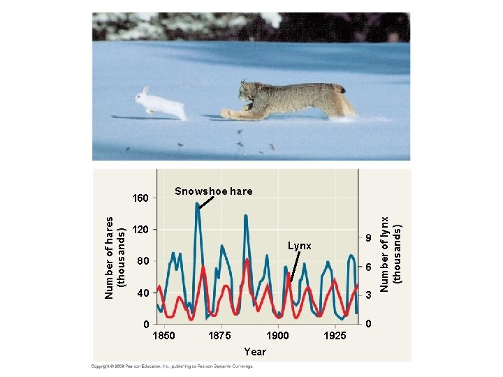
Population Cycles: Scientific Inquiry • Some populations undergo regular boom-andbust cycles. • Lynx populations follow the 10 year boom-andbust cycle of hare populations. • Three hypotheses have been proposed to explain the hare’s 10 -year interval. Copyright © 2008 Pearson Education, Inc. , publishing as Pearson Benjamin Cummings

Snowshoe hare 120 9 Lynx 80 6 40 3 0 0 1850 1875 1900 Year 1925 Number of lynx (thousands) Number of hares (thousands) 160

• Hypothesis 1: The hare’s population cycle follows a cycle of winter food supply. • If this hypothesis is correct, then the cycles should stop if the food supply is increased. • Additional food was provided experimentally to a hare population, and the whole population increased in size but continued to cycle. • No hares appeared to have died of starvation. Copyright © 2008 Pearson Education, Inc. , publishing as Pearson Benjamin Cummings

• Hypothesis 2: The hare’s population cycle is driven by pressure from other predators. • In a study conducted by field ecologists, 90% of the hares were killed by predators. • These data support this second hypothesis. Copyright © 2008 Pearson Education, Inc. , publishing as Pearson Benjamin Cummings

• Hypothesis 3: The hare’s population cycle is linked to sunspot cycles. • Sunspot activity affects light quality, which in turn affects the quality of the hares’ food. • There is good correlation between sunspot activity and hare population size. • The results of all these experiments suggest that both predation and sunspot activity regulate hare numbers and that food availability plays a less important role. Copyright © 2008 Pearson Education, Inc. , publishing as Pearson Benjamin Cummings

Immigration, Emigration, and Metapopulations • Metapopulations are groups of populations linked by immigration and emigration. • High levels of immigration combined with higher survival can result in greater stability in populations. Copyright © 2008 Pearson Education, Inc. , publishing as Pearson Benjamin Cummings

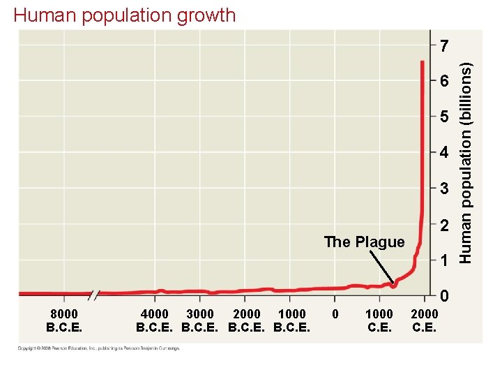
The human population is no longer growing exponentially but is still increasing rapidly • No population can grow indefinitely, and humans are no exception. • The human population increased relatively slowly until about 1650 and then began to grow exponentially. • Though the global population is still growing, the rate of growth began to slow during the 1960 s. • Most of the current global population growth is concentrated in developing countries. Copyright © 2008 Pearson Education, Inc. , publishing as Pearson Benjamin Cummings

Human population growth 6 5 4 3 2 The Plague 1 0 8000 B. C. E. 4000 3000 2000 1000 B. C. E. 0 1000 C. E. 2000 C. E. Human population (billions) 7

Regional Patterns of Population Change • To maintain population stability, a regional human population can exist in one of two configurations: – Zero population growth = High birth rate – High death rate – Zero population growth = Low birth rate – Low death rate • The demographic transition is the move from the first state toward the second state. Copyright © 2008 Pearson Education, Inc. , publishing as Pearson Benjamin Cummings

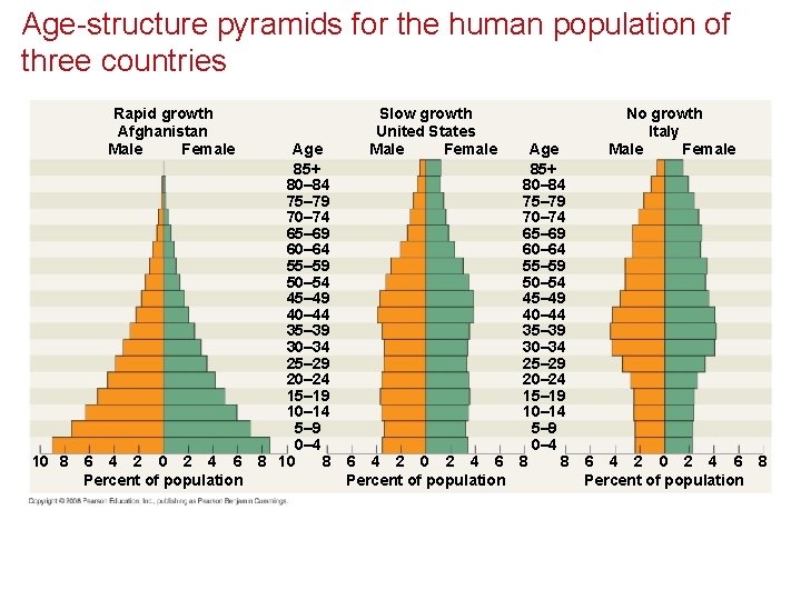
Age Structure • One important demographic factor in present and future growth trends is a country’s age structure. • Age structure is the relative number of individuals at each age. • Age structure diagrams can predict a population’s growth trends. • They can illuminate social conditions and help us plan for the future. Copyright © 2008 Pearson Education, Inc. , publishing as Pearson Benjamin Cummings

Age-structure pyramids for the human population of three countries Rapid growth Afghanistan Male Female 10 8 6 4 2 0 2 4 6 Percent of population Age 85+ 80– 84 75– 79 70– 74 65– 69 60– 64 55– 59 50– 54 45– 49 40– 44 35– 39 30– 34 25– 29 20– 24 15– 19 10– 14 5– 9 0– 4 8 10 8 Slow growth United States Male Female 6 4 2 0 2 4 6 Percent of population Age 85+ 80– 84 75– 79 70– 74 65– 69 60– 64 55– 59 50– 54 45– 49 40– 44 35– 39 30– 34 25– 29 20– 24 15– 19 10– 14 5– 9 0– 4 8 8 No growth Italy Male Female 6 4 2 0 2 4 6 8 Percent of population

Estimates of Earth’s Carrying Capacity • How many humans can the biosphere support? • The carrying capacity of Earth for humans is uncertain. • The average estimate is 10– 15 billion. Copyright © 2008 Pearson Education, Inc. , publishing as Pearson Benjamin Cummings

Limits on Human Population Size • The ecological footprint concept summarizes the aggregate land water area needed to sustain the people of a nation. • It is one measure of how close we are to the carrying capacity of Earth. • Countries vary greatly in footprint size and available ecological capacity. • Our carrying capacity could potentially be limited by food, space, nonrenewable resources, or buildup of wastes. Copyright © 2008 Pearson Education, Inc. , publishing as Pearson Benjamin Cummings

Population size (N) Review: Population Growth Curve K = carrying capacity K–N d. N = rmax N dt K Number of generations

You should now be able to: 1. Define and distinguish between the following sets of terms: density and dispersion; clumped dispersion, uniform dispersion, and random dispersion; life table and reproductive table; Type I, Type II, and Type III survivorship curves; semelparity and iteroparity; r-selected populations and K-selected populations. 2. Explain how ecologists may estimate the density of a species. Copyright © 2008 Pearson Education, Inc. , publishing as Pearson Benjamin Cummings

3. Explain how limited resources and trade-offs may affect life histories. 4. Compare the exponential and logistic models of population growth. 5. Explain how density-dependent and densityindependent factors may affect population growth. 6. Explain how biotic and abiotic factors may work together to control a population’s growth. Copyright © 2008 Pearson Education, Inc. , publishing as Pearson Benjamin Cummings