Chapter 5 Trees Instructors C Y Tang and

Chapter 5 Trees Instructors: C. Y. Tang and J. S. Roger Jang All the material are integrated from the textbook "Fundamentals of Data Structures in C" and some supplement from the slides of Prof. Hsin-Hsi Chen (NTU).

Outline (1) n n Introduction (5. 1) Binary Trees (5. 2) n n n Binary Tree Traversals (5. 3) Additional Binary Tree Operations (5. 4) Threaded Binary Trees (5. 5) Heaps (5. 6) & (Chapter 9) Binary Search Trees (5. 7)

Outline (2) n n n Selection Trees (5. 8) Forests (5. 9) Set Representation (5. 10) Counting Binary Trees (5. 11) References & Exercises

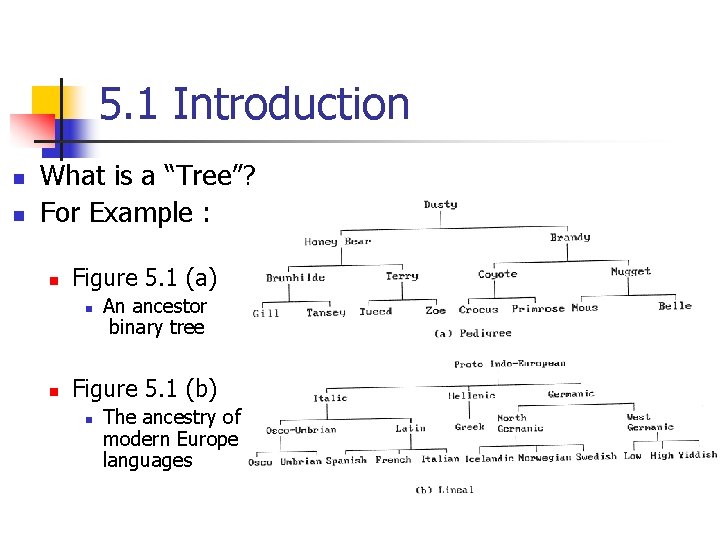
5. 1 Introduction n n What is a “Tree”? For Example : n Figure 5. 1 (a) n n An ancestor binary tree Figure 5. 1 (b) n The ancestry of modern Europe languages

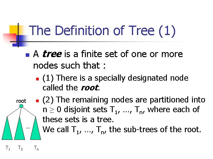
The Definition of Tree (1) n A tree is a finite set of one or more nodes such that : n root n … T 1 T 2 Tn (1) There is a specially designated node called the root. (2) The remaining nodes are partitioned into n ≥ 0 disjoint sets T 1, …, Tn, where each of these sets is a tree. We call T 1, …, Tn, the sub-trees of the root.

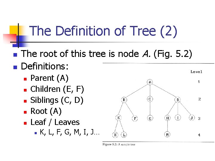
The Definition of Tree (2) n n The root of this tree is node A. (Fig. 5. 2) Definitions: n n n Parent (A) Children (E, F) Siblings (C, D) Root (A) Leaf / Leaves n K, L, F, G, M, I, J…

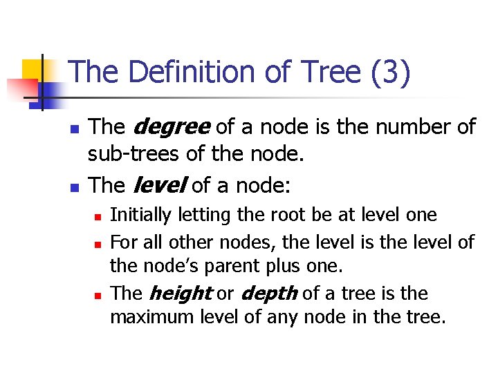
The Definition of Tree (3) n n The degree of a node is the number of sub-trees of the node. The level of a node: n n n Initially letting the root be at level one For all other nodes, the level is the level of the node’s parent plus one. The height or depth of a tree is the maximum level of any node in the tree.

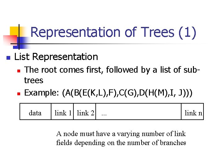
Representation of Trees (1) n List Representation n n The root comes first, followed by a list of subtrees Example: (A(B(E(K, L), F), C(G), D(H(M), I, J))) data link 1 link 2. . . link n A node must have a varying number of link fields depending on the number of branches

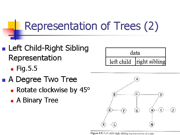
Representation of Trees (2) n Left Child-Right Sibling Representation n n Fig. 5. 5 A Degree Two Tree n n Rotate clockwise by 45° A Binary Tree data left child right sibling

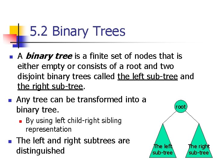
5. 2 Binary Trees n n A binary tree is a finite set of nodes that is either empty or consists of a root and two disjoint binary trees called the left sub-tree and the right sub-tree. Any tree can be transformed into a binary tree. n n root By using left child-right sibling representation The left and right subtrees are distinguished The left sub-tree The right sub-tree

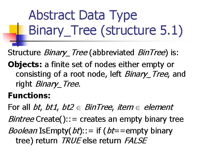
Abstract Data Type Binary_Tree (structure 5. 1) Structure Binary_Tree (abbreviated Bin. Tree) is: Objects: a finite set of nodes either empty or consisting of a root node, left Binary_Tree, and right Binary_Tree. Functions: For all bt, bt 1, bt 2 Bin. Tree, item element Bintree Create(): : = creates an empty binary tree Boolean Is. Empty(bt): : = if (bt==empty binary tree) return TRUE else return FALSE

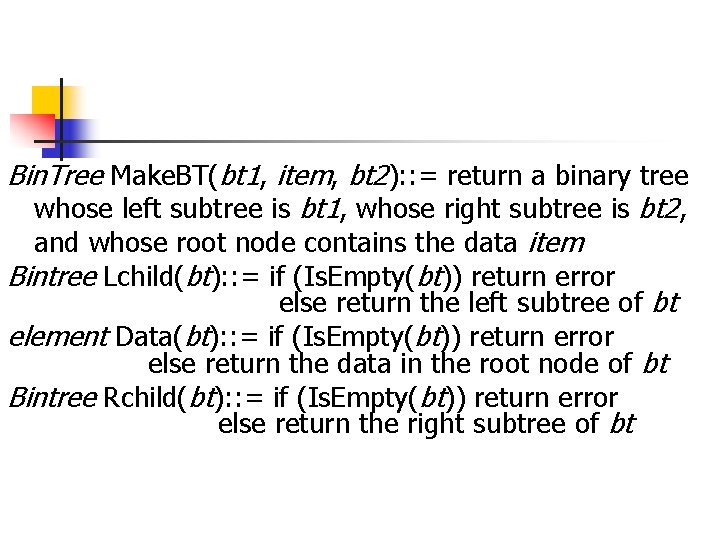
Bin. Tree Make. BT(bt 1, item, bt 2): : = return a binary tree whose left subtree is bt 1, whose right subtree is bt 2, and whose root node contains the data item Bintree Lchild(bt): : = if (Is. Empty(bt)) return error else return the left subtree of bt element Data(bt): : = if (Is. Empty(bt)) return error else return the data in the root node of bt Bintree Rchild(bt): : = if (Is. Empty(bt)) return error else return the right subtree of bt

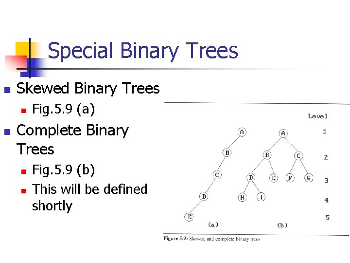
Special Binary Trees n Skewed Binary Trees n n Fig. 5. 9 (a) Complete Binary Trees n n Fig. 5. 9 (b) This will be defined shortly

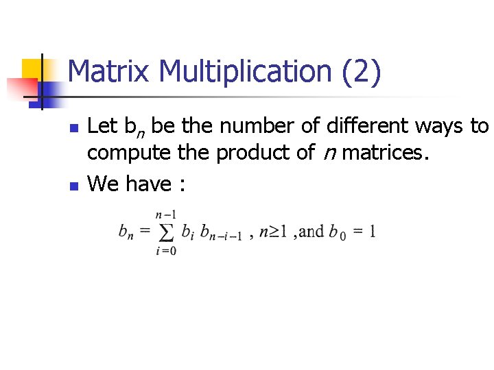
Properties of Binary Trees (1) n Lemma 5. 1 [Maximum number of nodes] : n n (1) The maximum number of nodes on level i of a binary tree is 2 i -1, i ≥ 1. (2) The maximum number of nodes in a binary tree of depth k is is 2 k -1, k ≥ 1. The proof is by induction on i. Lemma 5. 2 : n For any nonempty binary tree, T, if n 0 is the number of leaf nodes and n 2 the number of nodes of degree 2, then n 0 = n 2 +1.

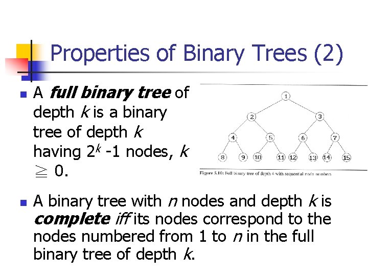
Properties of Binary Trees (2) n n A full binary tree of depth k is a binary tree of depth k having 2 k -1 nodes, k ≧ 0. A binary tree with n nodes and depth k is complete iff its nodes correspond to the nodes numbered from 1 to n in the full binary tree of depth k.

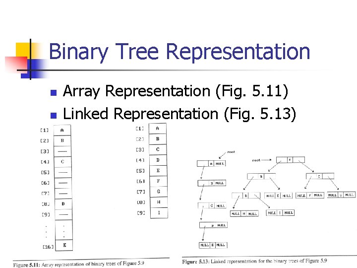
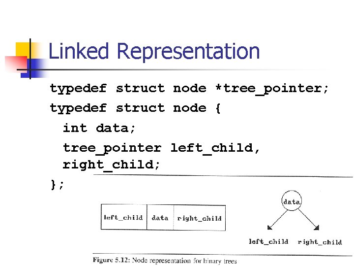
Binary Tree Representation n n Array Representation (Fig. 5. 11) Linked Representation (Fig. 5. 13)

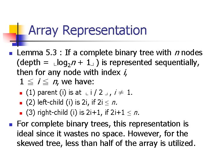
Array Representation n Lemma 5. 3 : If a complete binary tree with n nodes (depth = └log 2 n + 1┘) is represented sequentially, then for any node with index i, 1 ≦ i ≦ n, we have: n n (1) parent (i) is at └ i / 2 ┘, i ≠ 1. (2) left-child (i) is 2 i, if 2 i ≤ n. (3) right-child (i) is 2 i+1, if 2 i+1 ≤ n. For complete binary trees, this representation is ideal since it wastes no space. However, for the skewed tree, less than half of the array is utilized.

Linked Representation typedef struct node *tree_pointer; typedef struct node { int data; tree_pointer left_child, right_child; };

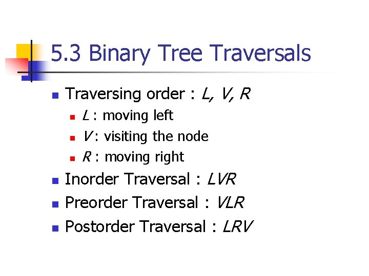
5. 3 Binary Tree Traversals n Traversing order : L, V, R n n n L : moving left V : visiting the node R : moving right Inorder Traversal : LVR Preorder Traversal : VLR Postorder Traversal : LRV

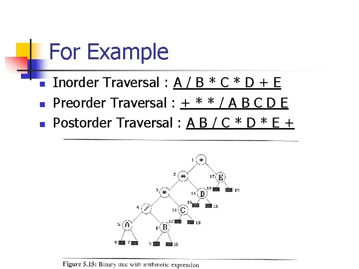
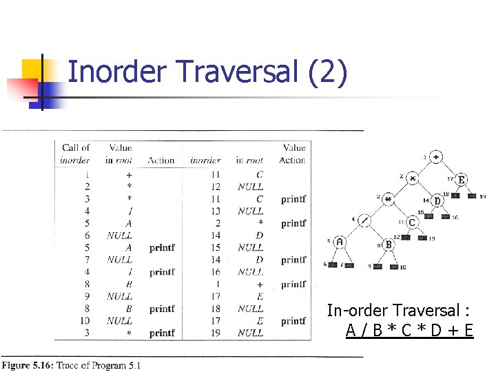
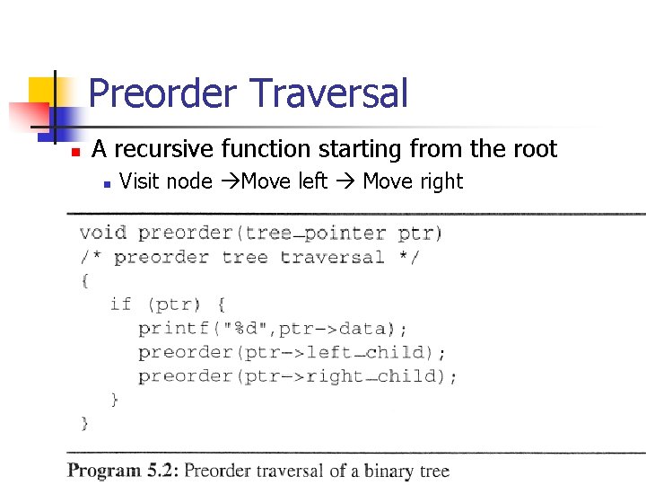
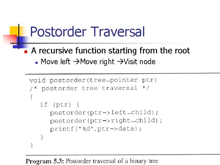
For Example n n n Inorder Traversal : A / B * C * D + E Preorder Traversal : + * * / A B C D E Postorder Traversal : A B / C * D * E +

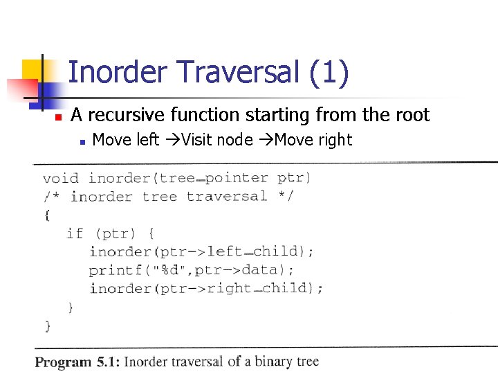
Inorder Traversal (1) n A recursive function starting from the root n Move left Visit node Move right

Inorder Traversal (2) In-order Traversal : A/B*C*D+E

Preorder Traversal n A recursive function starting from the root n Visit node Move left Move right

Postorder Traversal n A recursive function starting from the root n Move left Move right Visit node

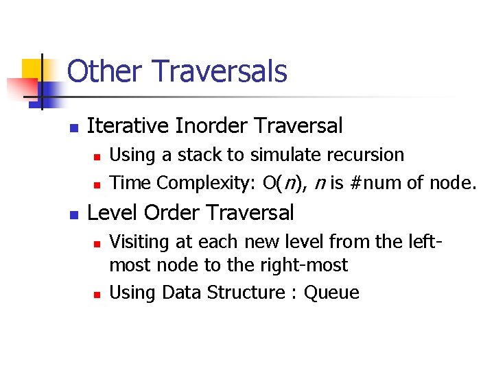
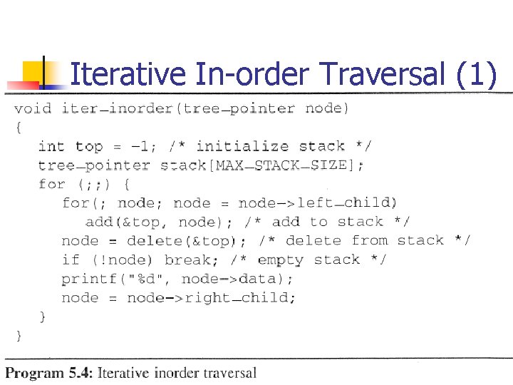
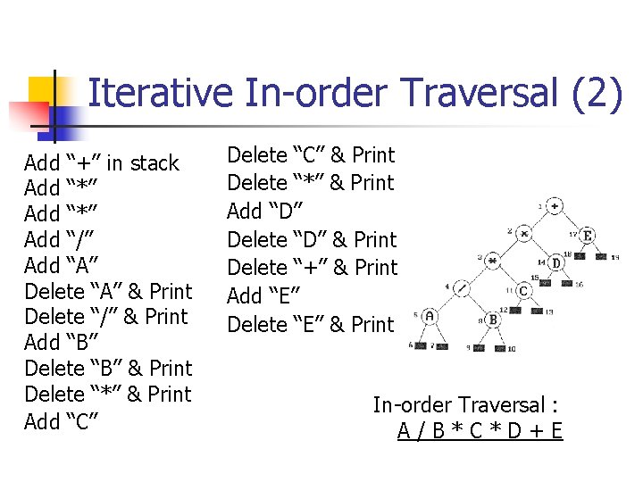
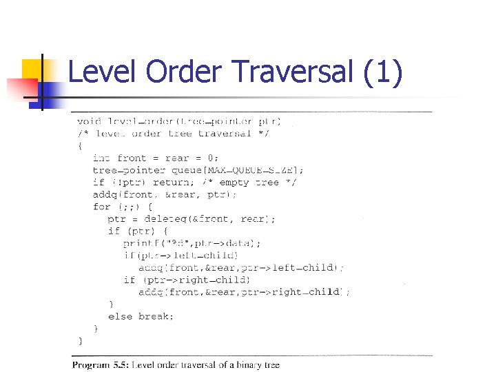
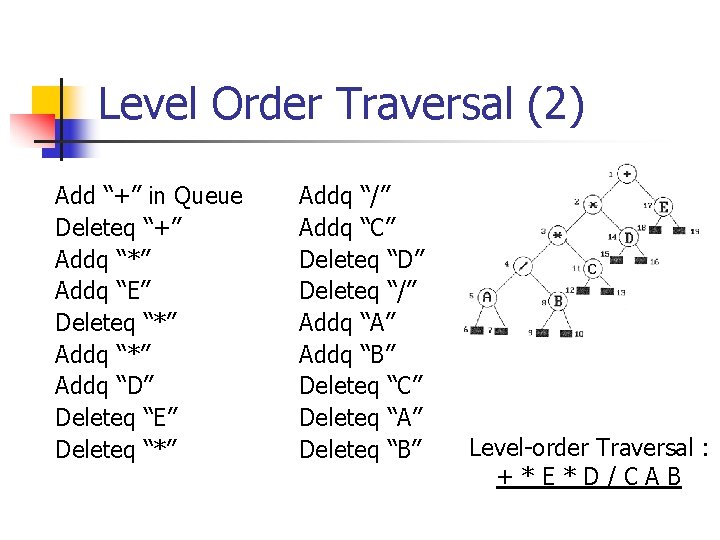
Other Traversals n Iterative Inorder Traversal n n n Using a stack to simulate recursion Time Complexity: O(n), n is #num of node. Level Order Traversal n n Visiting at each new level from the leftmost node to the right-most Using Data Structure : Queue

Iterative In-order Traversal (1)

Iterative In-order Traversal (2) Add “+” in stack Add “*” Add “/” Add “A” Delete “A” & Print Delete “/” & Print Add “B” Delete “B” & Print Delete “*” & Print Add “C” Delete “C” & Print Delete “*” & Print Add “D” Delete “D” & Print Delete “+” & Print Add “E” Delete “E” & Print In-order Traversal : A/B*C*D+E

Level Order Traversal (1)

Level Order Traversal (2) Add “+” in Queue Deleteq “+” Addq “*” Addq “E” Deleteq “*” Addq “D” Deleteq “E” Deleteq “*” Addq “/” Addq “C” Deleteq “D” Deleteq “/” Addq “A” Addq “B” Deleteq “C” Deleteq “A” Deleteq “B” Level-order Traversal : +*E*D/CAB

5. 4 Additional Binary Tree Operations n Copying Binary Trees n n Testing for Equality of Binary Trees n n Program 5. 6 Program 5. 7 The Satisfiability Problem (SAT)

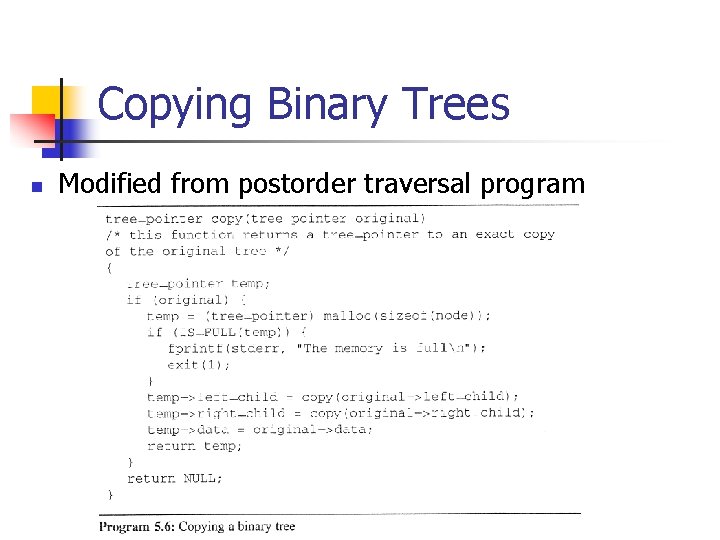
Copying Binary Trees n Modified from postorder traversal program

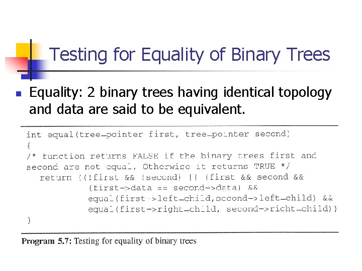
Testing for Equality of Binary Trees n Equality: 2 binary trees having identical topology and data are said to be equivalent.

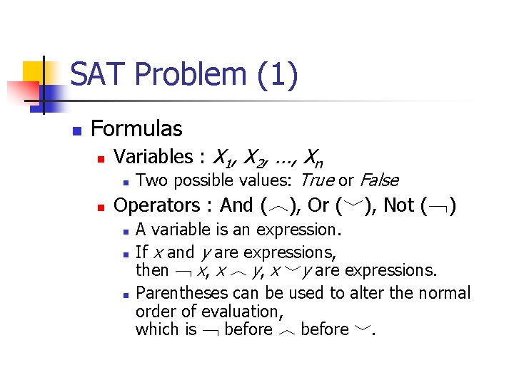
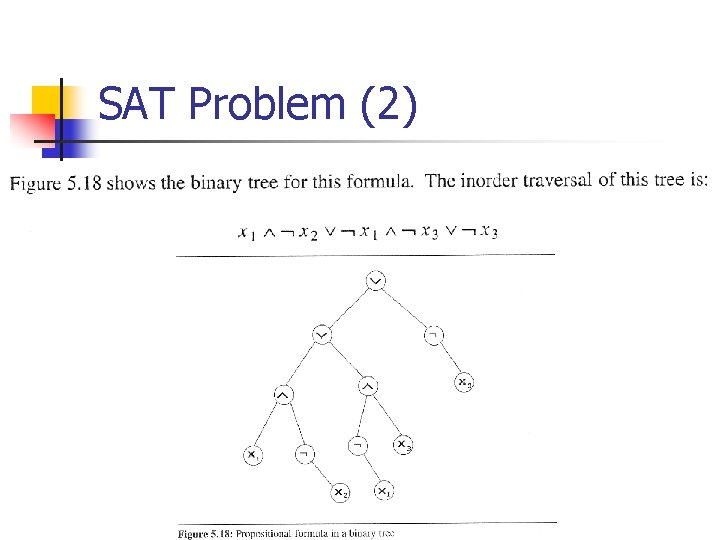
SAT Problem (1) n Formulas n Variables : X 1, X 2, …, Xn n n Two possible values: True or False Operators : And (︿), Or (﹀), Not (﹁) n n n A variable is an expression. If x and y are expressions, then ﹁ x, x ︿ y, x ﹀y are expressions. Parentheses can be used to alter the normal order of evaluation, which is ﹁ before ︿ before ﹀.

SAT Problem (2)

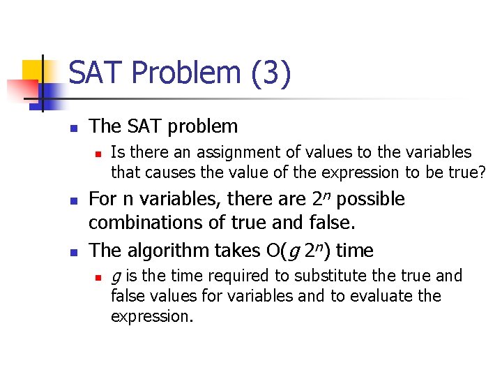
SAT Problem (3) n The SAT problem n n n Is there an assignment of values to the variables that causes the value of the expression to be true? For n variables, there are 2 n possible combinations of true and false. The algorithm takes O(g 2 n) time n g is the time required to substitute the true and false values for variables and to evaluate the expression.

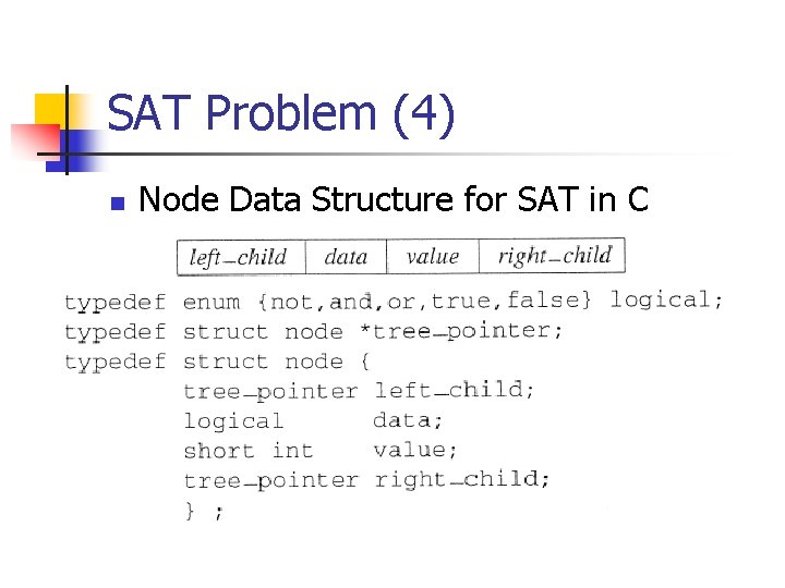
SAT Problem (4) n Node Data Structure for SAT in C

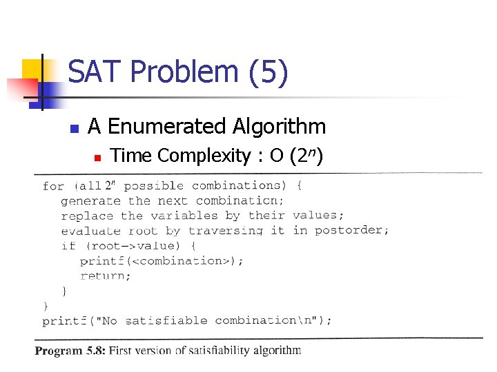
SAT Problem (5) n A Enumerated Algorithm n Time Complexity : O (2 n)

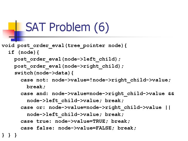
SAT Problem (6) void post_order_eval(tree_pointer node){ if (node){ post_order_eval(node->left_child); post_order_eval(node->right_child); switch(node->data){ case not: node->value=!node->right_child->value; break; case and: node->value=node->right_child->value && node->left_child->value; break; case or: node->value=node->right_child->value || node->left_child->value; break; case true: node->value=TRUE; break; case false: node->value=FALSE; break; } } }

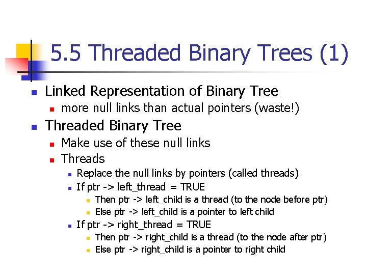
5. 5 Threaded Binary Trees (1) n Linked Representation of Binary Tree n n more null links than actual pointers (waste!) Threaded Binary Tree n n Make use of these null links Threads n n Replace the null links by pointers (called threads) If ptr -> left_thread = TRUE n n n Then ptr -> left_child is a thread (to the node before ptr) Else ptr -> left_child is a pointer to left child If ptr -> right_thread = TRUE n n Then ptr -> right_child is a thread (to the node after ptr) Else ptr -> right_child is a pointer to right child

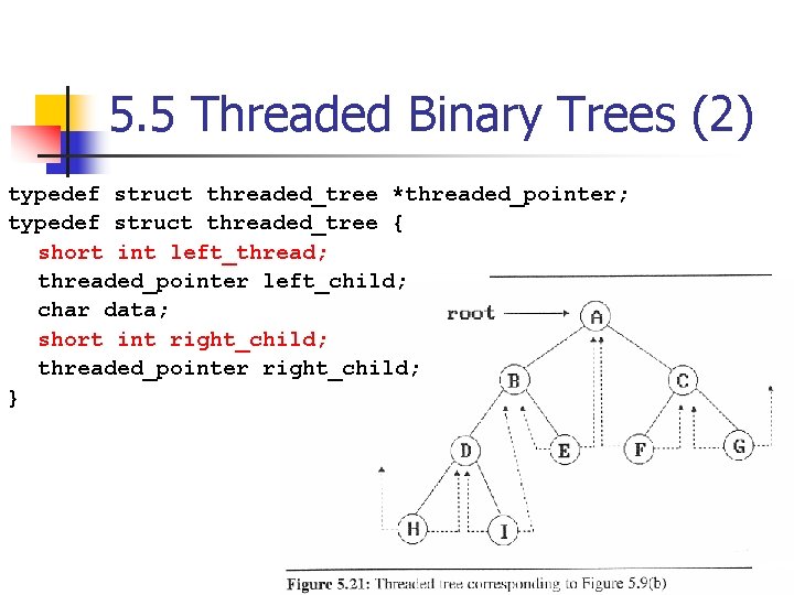
5. 5 Threaded Binary Trees (2) typedef struct threaded_tree *threaded_pointer; typedef struct threaded_tree { short int left_thread; threaded_pointer left_child; char data; short int right_child; threaded_pointer right_child; }

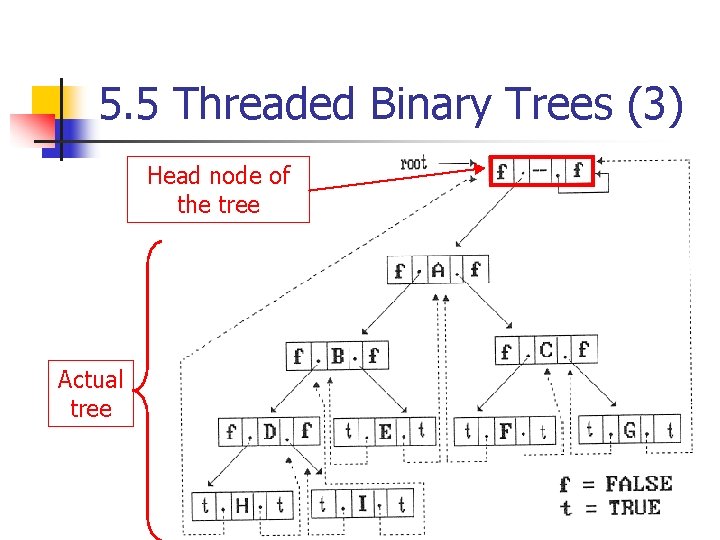
5. 5 Threaded Binary Trees (3) Head node of the tree Actual tree

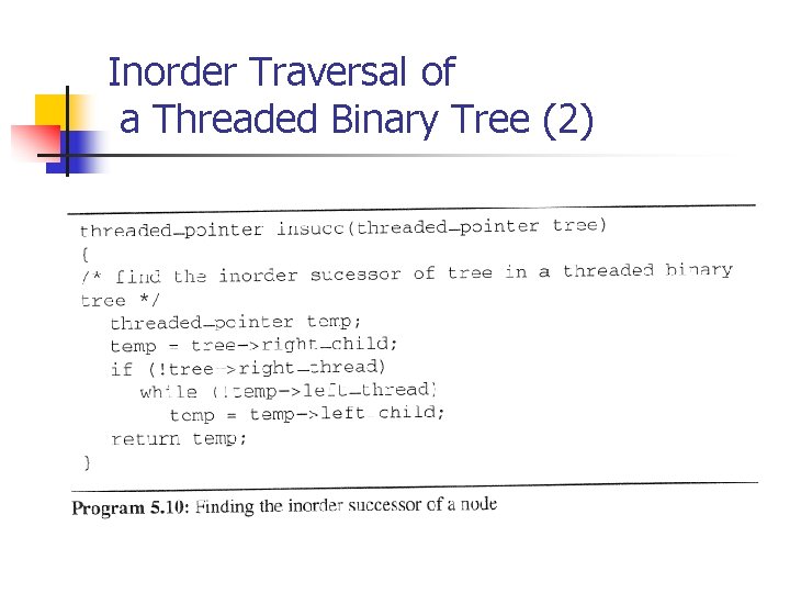
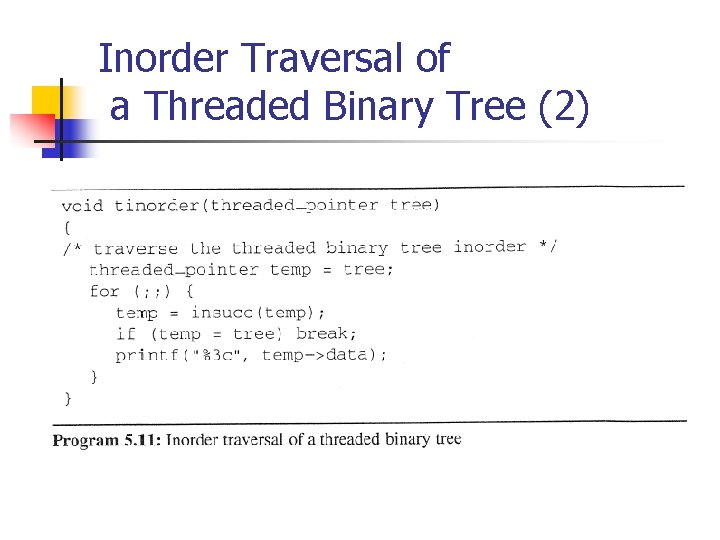
Inorder Traversal of a Threaded Binary Tree (1) n n Threads simplify inorder traversal algorithm An easy O(n) algorithm (Program 5. 11. ) n For any node, ptr, in a threaded binary tree n If ptr -> right_thread = TRUE n n Else (Otherwise, ptr -> right_thread = FALSE) n n The inorder successor of ptr = ptr -> right_child Follow a path of left_child links from the right_child of ptr until finding a node with left_Thread = TRUE Function insucc (Program 5. 10. ) n Finds the inorder successor of any node (without using a stack)

Inorder Traversal of a Threaded Binary Tree (2)

Inorder Traversal of a Threaded Binary Tree (2)

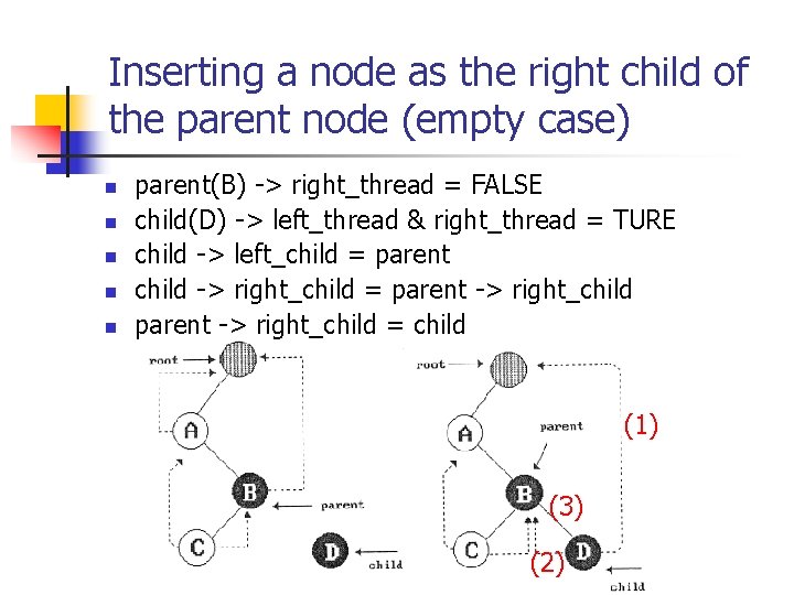
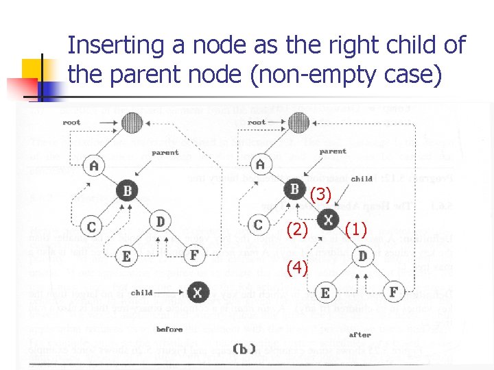
Inserting a Node into a Threaded Binary Tree n Insert a new node as a child of a parent node n n n Insert as a left child (left as an exercise) Insert as a right child (see examples 1 and 2) Is the original child node an empty subtree? n Empty child node (parent -> child_thread = TRUE) n n See example 1 Non-empty child node (parent -> child_thread = FALSE) n See example 2

Inserting a node as the right child of the parent node (empty case) n n n parent(B) -> right_thread = FALSE child(D) -> left_thread & right_thread = TURE child -> left_child = parent child -> right_child = parent -> right_child = child (1) (3) (2)

Inserting a node as the right child of the parent node (non-empty case) (3) (2) (4) (1)

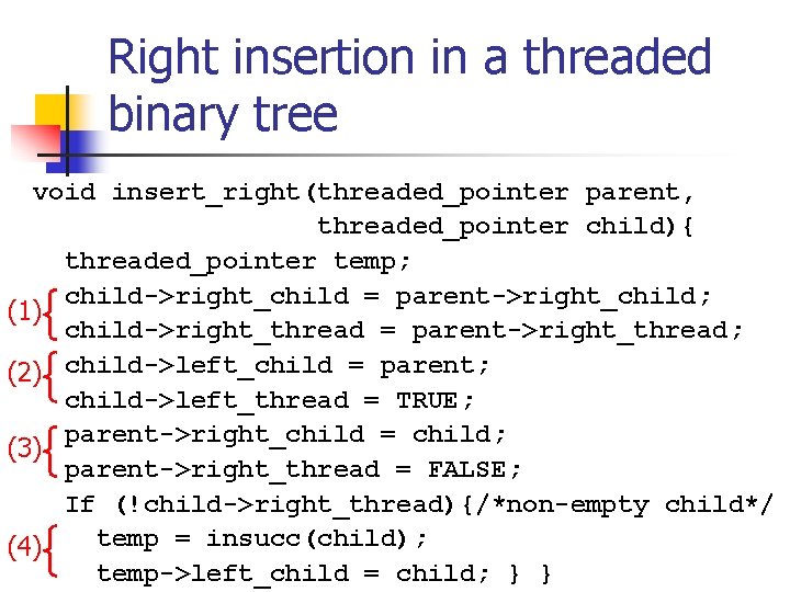
Right insertion in a threaded binary tree void insert_right(threaded_pointer parent, threaded_pointer child){ threaded_pointer temp; child->right_child = parent->right_child; (1) child->right_thread = parent->right_thread; (2) child->left_child = parent; child->left_thread = TRUE; parent->right_child = child; (3) parent->right_thread = FALSE; If (!child->right_thread){/*non-empty child*/ temp = insucc(child); (4) temp->left_child = child; } }

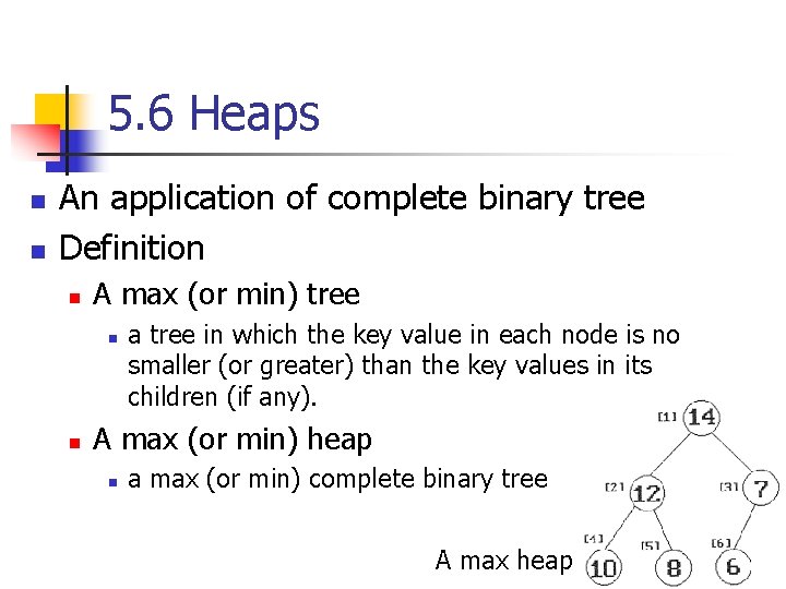
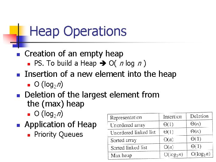
5. 6 Heaps n n An application of complete binary tree Definition n A max (or min) tree n n a tree in which the key value in each node is no smaller (or greater) than the key values in its children (if any). A max (or min) heap n a max (or min) complete binary tree A max heap

Heap Operations n Creation of an empty heap n n Insertion of a new element into the heap n n O (log 2 n) Deletion of the largest element from the (max) heap n n PS. To build a Heap O( n log n ) O (log 2 n) Application of Heap n Priority Queues

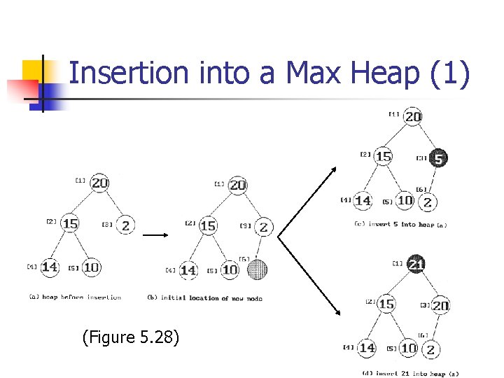
Insertion into a Max Heap (1) (Figure 5. 28)

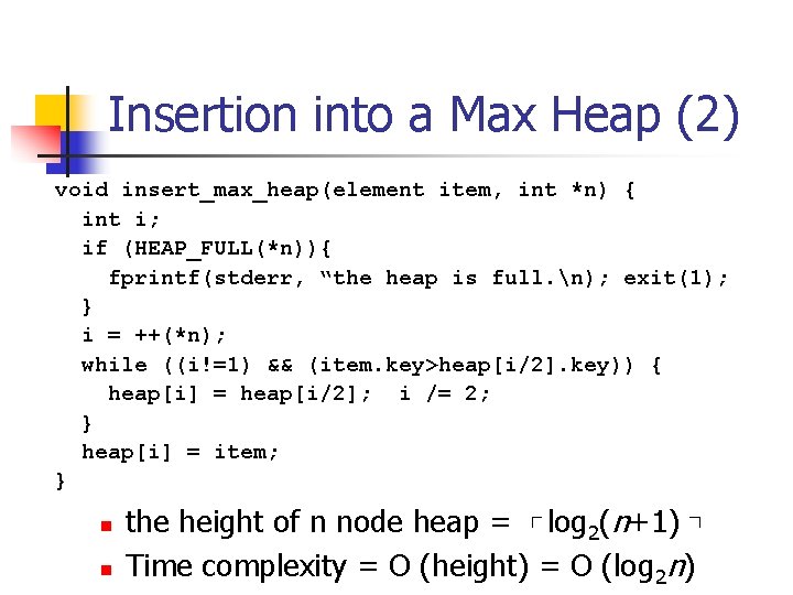
Insertion into a Max Heap (2) void insert_max_heap(element item, int *n) { int i; if (HEAP_FULL(*n)){ fprintf(stderr, “the heap is full. n); exit(1); } i = ++(*n); while ((i!=1) && (item. key>heap[i/2]. key)) { heap[i] = heap[i/2]; i /= 2; } heap[i] = item; } n n the height of n node heap = ┌ log 2(n+1) ┐ Time complexity = O (height) = O (log 2 n)

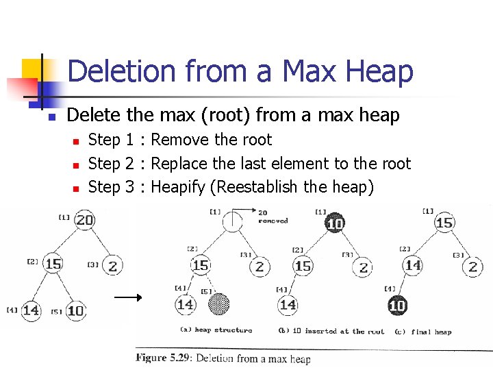
Deletion from a Max Heap n Delete the max (root) from a max heap n n n Step 1 : Remove the root Step 2 : Replace the last element to the root Step 3 : Heapify (Reestablish the heap)

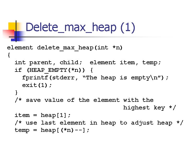
Delete_max_heap (1) element delete_max_heap(int *n) { int parent, child; element item, temp; if (HEAP_EMPTY(*n)) { fprintf(stderr, “The heap is emptyn”); exit(1); } /* save value of the element with the highest key */ item = heap[1]; /* use last element in heap to adjust heap */ temp = heap[(*n)--];

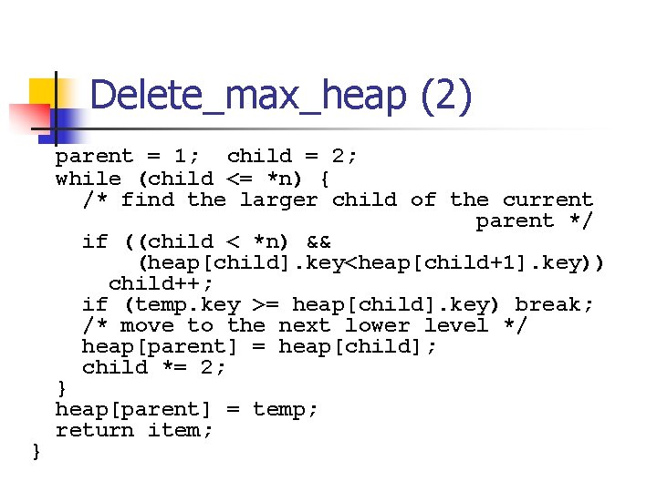
Delete_max_heap (2) } parent = 1; child = 2; while (child <= *n) { /* find the larger child of the current parent */ if ((child < *n) && (heap[child]. key<heap[child+1]. key)) child++; if (temp. key >= heap[child]. key) break; /* move to the next lower level */ heap[parent] = heap[child]; child *= 2; } heap[parent] = temp; return item;

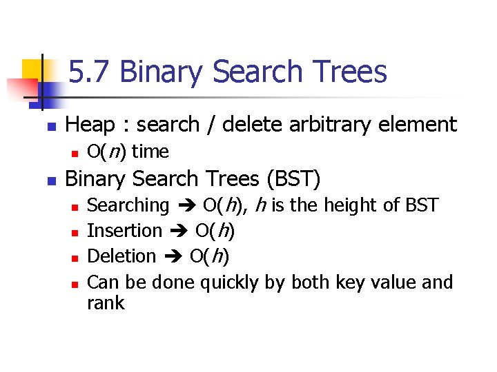
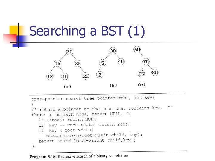
5. 7 Binary Search Trees n Heap : search / delete arbitrary element n n O(n) time Binary Search Trees (BST) n n Searching O(h), h is the height of BST Insertion O(h) Deletion O(h) Can be done quickly by both key value and rank

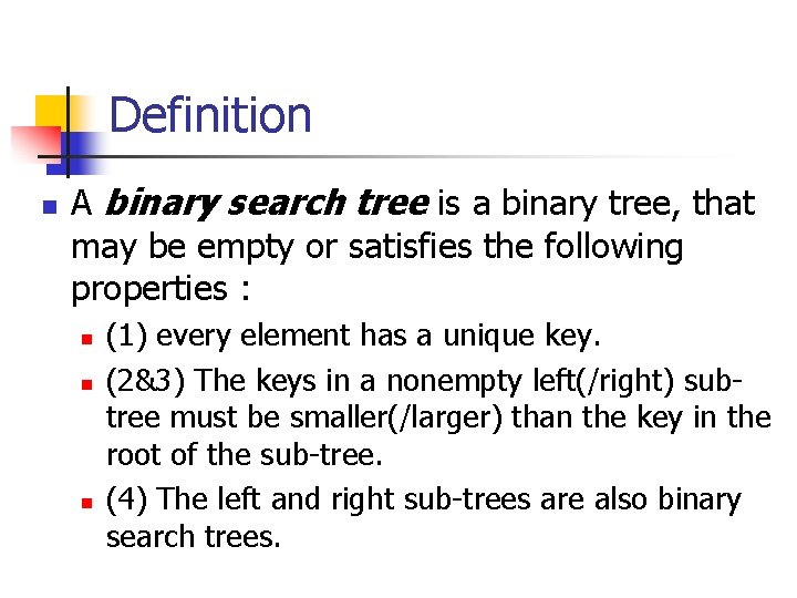
Definition n A binary search tree is a binary tree, that may be empty or satisfies the following properties : n n n (1) every element has a unique key. (2&3) The keys in a nonempty left(/right) subtree must be smaller(/larger) than the key in the root of the sub-tree. (4) The left and right sub-trees are also binary search trees.

Searching a BST (1)

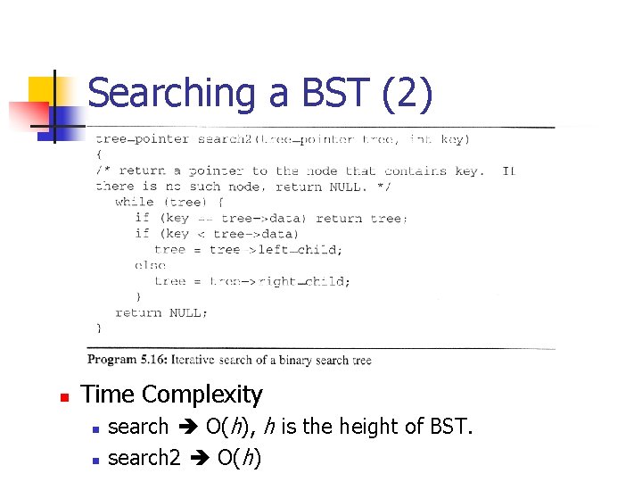
Searching a BST (2) n Time Complexity n n search O(h), h is the height of BST. search 2 O(h)

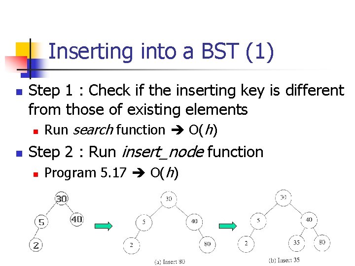
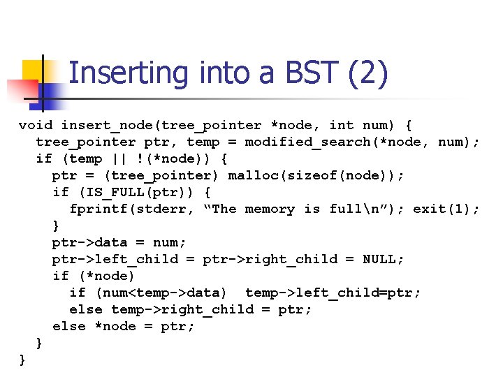
Inserting into a BST (1) n Step 1 : Check if the inserting key is different from those of existing elements n n Run search function O(h) Step 2 : Run insert_node function n Program 5. 17 O(h)

Inserting into a BST (2) void insert_node(tree_pointer *node, int num) { tree_pointer ptr, temp = modified_search(*node, num); if (temp || !(*node)) { ptr = (tree_pointer) malloc(sizeof(node)); if (IS_FULL(ptr)) { fprintf(stderr, “The memory is fulln”); exit(1); } ptr->data = num; ptr->left_child = ptr->right_child = NULL; if (*node) if (num<temp->data) temp->left_child=ptr; else temp->right_child = ptr; else *node = ptr; } }

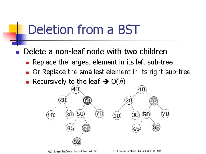
Deletion from a BST n Delete a non-leaf node with two children n Replace the largest element in its left sub-tree Or Replace the smallest element in its right sub-tree Recursively to the leaf O(h)

Height of a BST n The Height of the binary search tree is O(log 2 n), on the average. n n Worst case (skewed) O(h) = O(n) Balanced Search Trees n n With a worst case height of O(log 2 n) AVL Trees, 2 -3 Trees, Red-Black Trees n Chapter 10

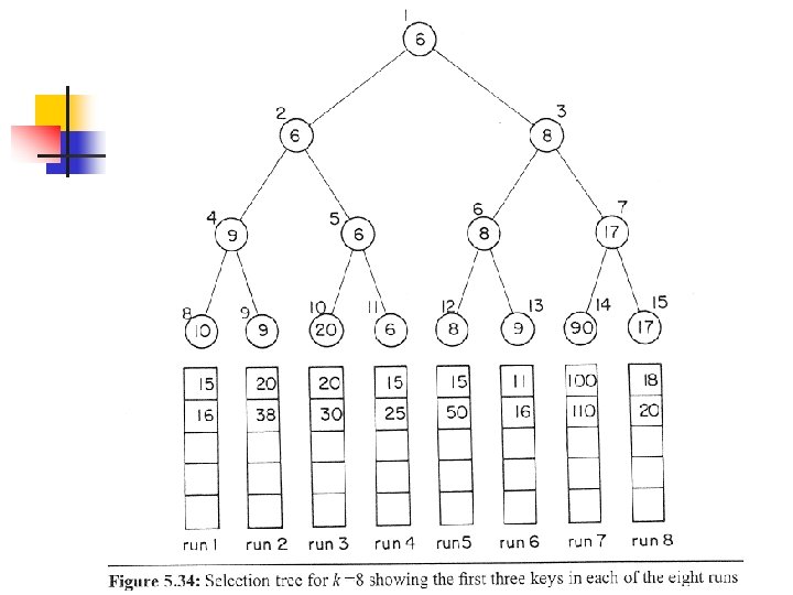
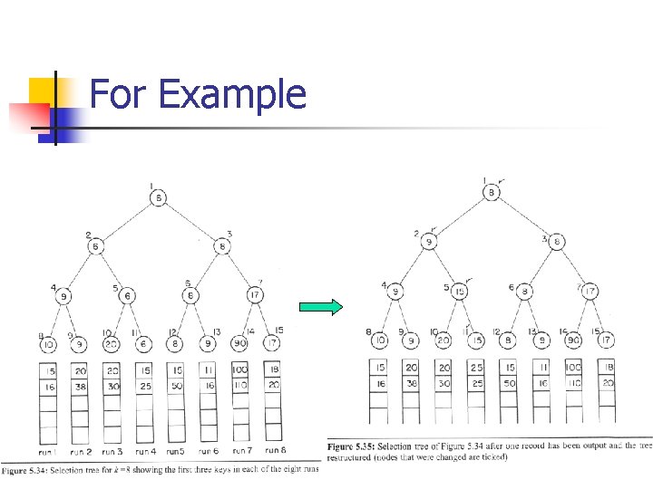
5. 8 Selection Trees n Application Problem n n n Merge k ordered sequences into a single ordered sequence Definition: A run is an ordered sequence Build a k-run Selection tree

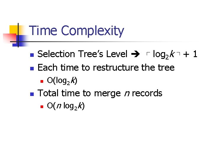
Time Complexity n n Selection Tree’s Level ┌ log 2 k ┐+ 1 Each time to restructure the tree n n O(log 2 k) Total time to merge n records n O(n log 2 k)

For Example

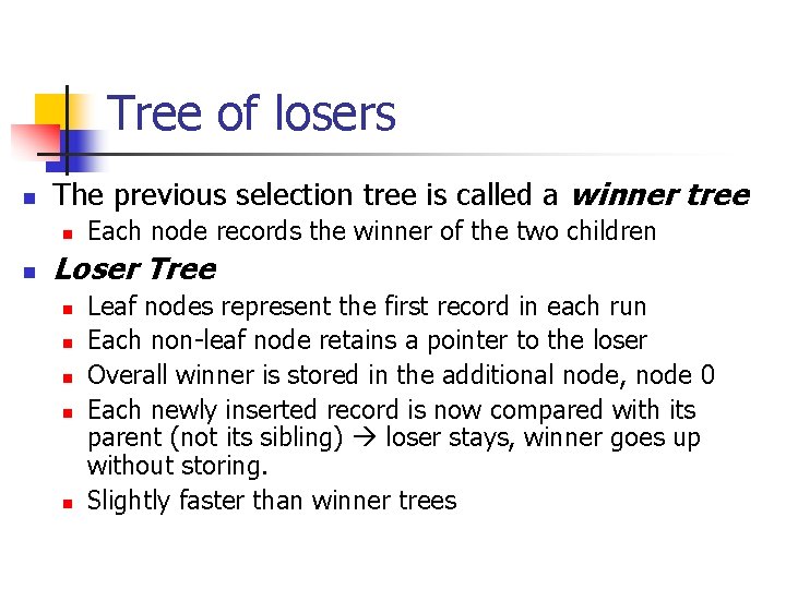
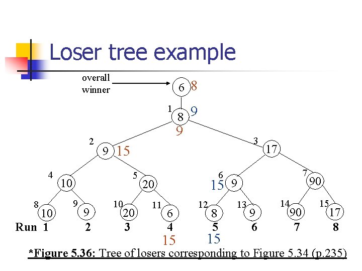
Tree of losers n The previous selection tree is called a winner tree n n Each node records the winner of the two children Loser Tree n n n Leaf nodes represent the first record in each run Each non-leaf node retains a pointer to the loser Overall winner is stored in the additional node, node 0 Each newly inserted record is now compared with its parent (not its sibling) loser stays, winner goes up without storing. Slightly faster than winner trees

Loser tree example overall winner 6 8 1 2 4 8 10 Run 1 9 10 9 2 3 9 15 5 9 8 9 10 20 3 17 7 6 15 9 20 11 6 4 15 12 8 5 15 13 9 6 14 90 7 90 15 17 8 *Figure 5. 36: Tree of losers corresponding to Figure 5. 34 (p. 235)

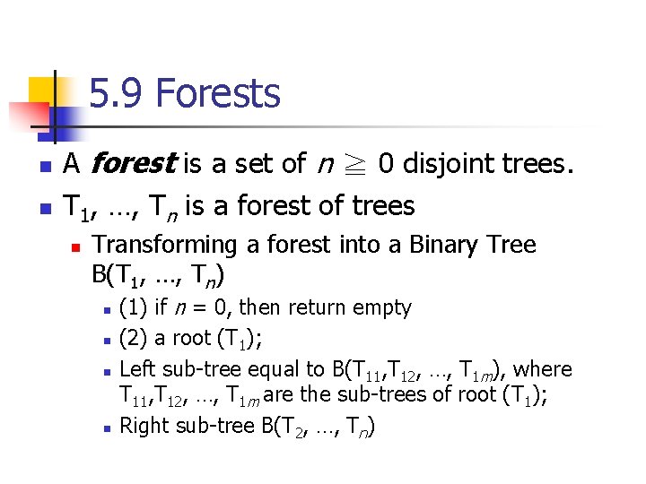
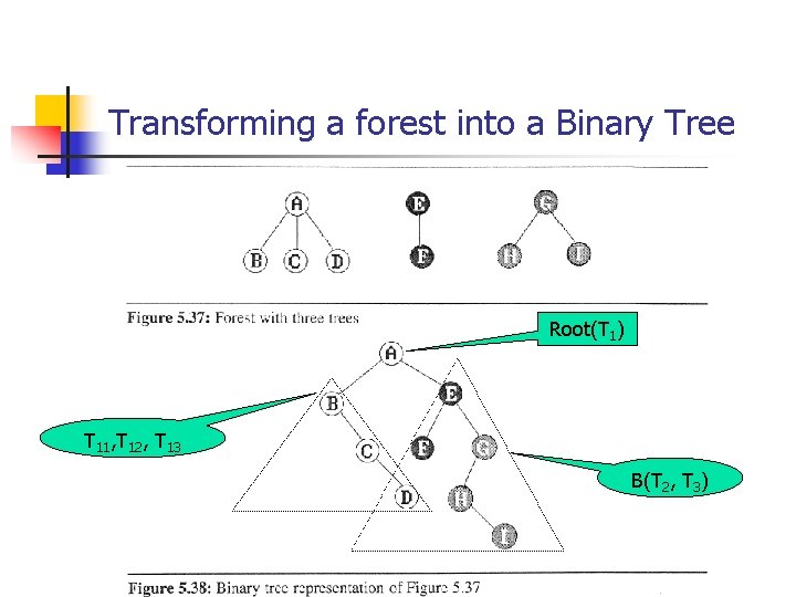
5. 9 Forests n n A forest is a set of n ≧ 0 disjoint trees. T 1, …, Tn is a forest of trees n Transforming a forest into a Binary Tree B(T 1, …, Tn) n n (1) if n = 0, then return empty (2) a root (T 1); Left sub-tree equal to B(T 11, T 12, …, T 1 m), where T 11, T 12, …, T 1 m are the sub-trees of root (T 1); Right sub-tree B(T 2, …, Tn)

Transforming a forest into a Binary Tree Root(T 1) T 11, T 12, T 13 B(T 2, T 3)

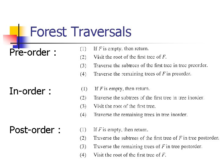
Forest Traversals Pre-order : In-order : Post-order :

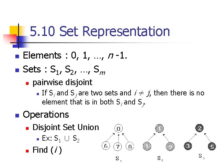
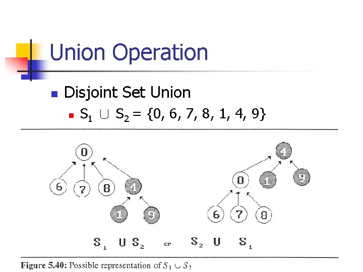
5. 10 Set Representation n n Elements : 0, 1, …, n -1. Sets : S 1, S 2, …, Sm n pairwise disjoint n n If Si and Sj are two sets and i ≠ j, then there is no element that is in both Si and Sj. Operations n Disjoint Set Union n n Ex: S 1 ∪ S 2 Find (i )

Union Operation n Disjoint Set Union n S 1 ∪ S 2 = {0, 6, 7, 8, 1, 4, 9}

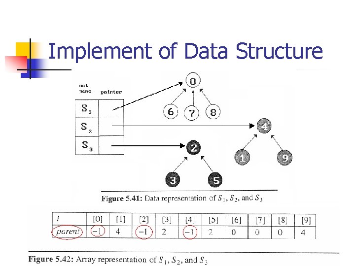
Implement of Data Structure

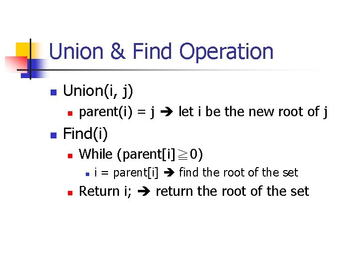
Union & Find Operation n Union(i, j) n n parent(i) = j let i be the new root of j Find(i) n While (parent[i]≧ 0) n n i = parent[i] find the root of the set Return i; return the root of the set

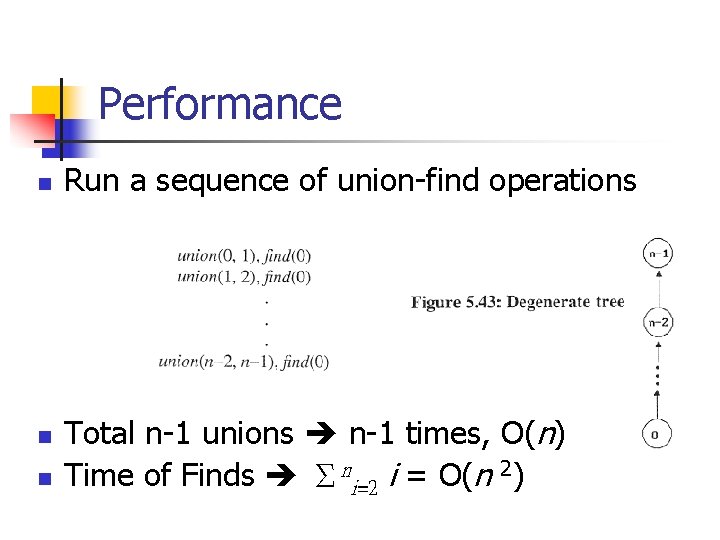
Performance n n n Run a sequence of union-find operations Total n-1 unions n-1 times, O(n) Time of Finds Σni=2 i = O(n 2)

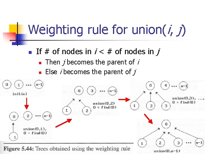
Weighting rule for union(i, j) n If # of nodes in i < # of nodes in j n n Then j becomes the parent of i Else i becomes the parent of j

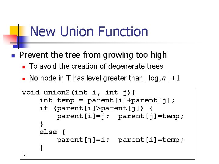
New Union Function n Prevent the tree from growing too high n To avoid the creation of degenerate trees n No node in T has level greater than log 2 n +1 void union 2(int i, int j){ int temp = parent[i]+parent[j]; if (parent[i]>parent[j]) { parent[i]=j; parent[j]=temp; } else { parent[j]=i; parent[i]=temp; } }

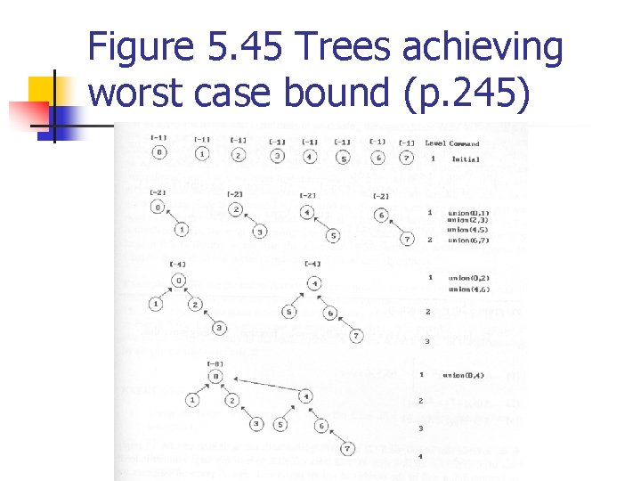
Figure 5. 45 Trees achieving worst case bound (p. 245)

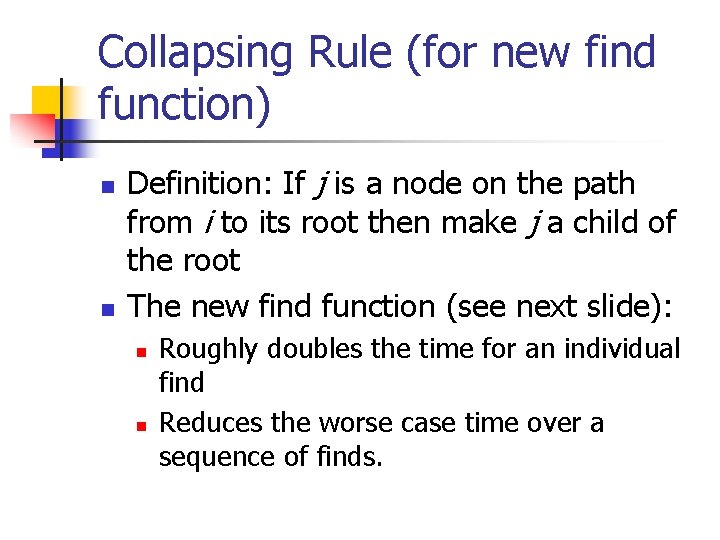
Collapsing Rule (for new find function) n n Definition: If j is a node on the path from i to its root then make j a child of the root The new find function (see next slide): n n Roughly doubles the time for an individual find Reduces the worse case time over a sequence of finds.

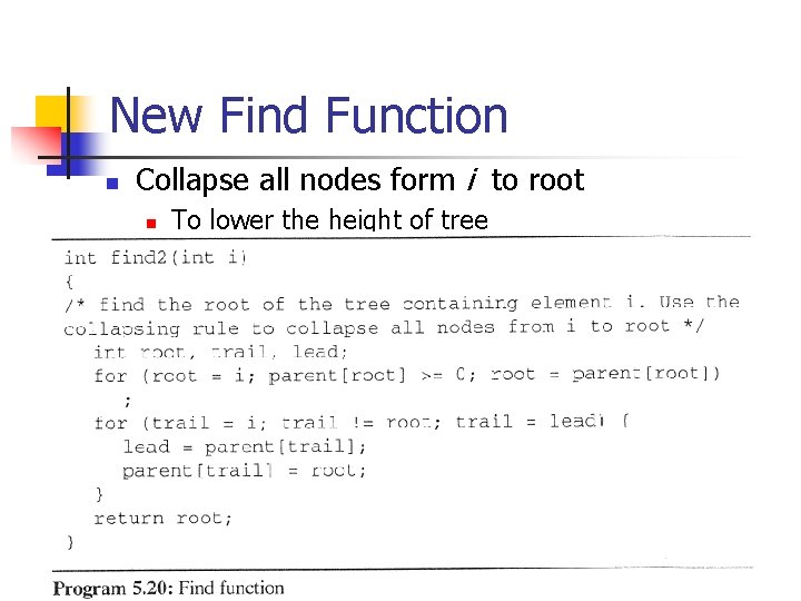
New Find Function n Collapse all nodes form i to root n To lower the height of tree

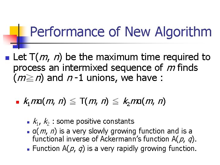
Performance of New Algorithm n Let T(m, n) be the maximum time required to process an intermixed sequence of m finds (m≧n) and n -1 unions, we have : n k 1 mα(m, n) ≦ T(m, n) ≦ k 2 mα(m, n) n n n k 1, k 2 : some positive constants α(m, n) is a very slowly growing function and is a functional inverse of Ackermann’s function A(p, q). Function A(p, q) is a very rapidly growing function.

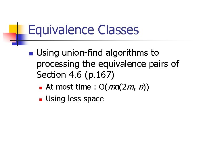
Equivalence Classes n Using union-find algorithms to processing the equivalence pairs of Section 4. 6 (p. 167) n n At most time : O(mα(2 m, n)) Using less space

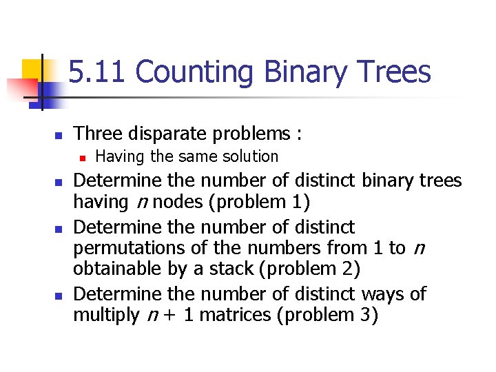
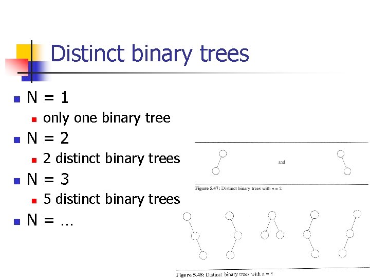
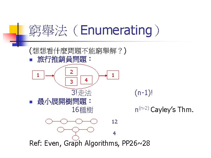
5. 11 Counting Binary Trees n Three disparate problems : n n Having the same solution Determine the number of distinct binary trees having n nodes (problem 1) Determine the number of distinct permutations of the numbers from 1 to n obtainable by a stack (problem 2) Determine the number of distinct ways of multiply n + 1 matrices (problem 3)

Distinct binary trees n N=1 n n N=2 n n 2 distinct binary trees N=3 n n only one binary tree 5 distinct binary trees N=…

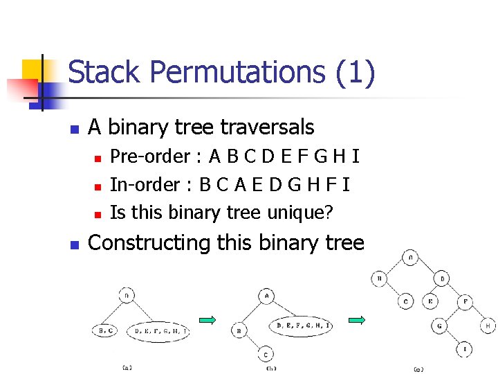
Stack Permutations (1) n A binary tree traversals n n Pre-order : A B C D E F G H I In-order : B C A E D G H F I Is this binary tree unique? Constructing this binary tree

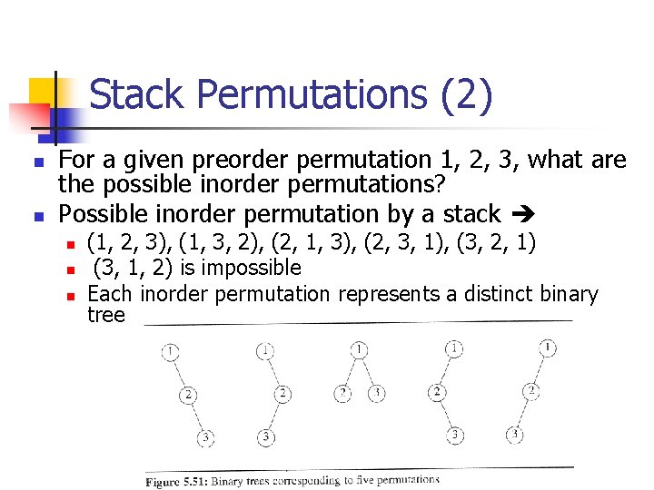
Stack Permutations (2) n n For a given preorder permutation 1, 2, 3, what are the possible inorder permutations? Possible inorder permutation by a stack n n n (1, 2, 3), (1, 3, 2), (2, 1, 3), (2, 3, 1), (3, 2, 1) (3, 1, 2) is impossible Each inorder permutation represents a distinct binary tree

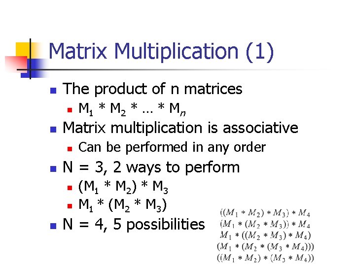
Matrix Multiplication (1) n The product of n matrices n n Matrix multiplication is associative n n Can be performed in any order N = 3, 2 ways to perform n n n M 1 * M 2 * … * M n (M 1 * M 2) * M 3 M 1 * (M 2 * M 3) N = 4, 5 possibilities

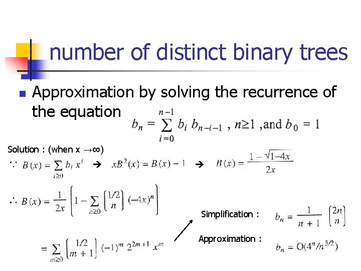
Matrix Multiplication (2) n n Let bn be the number of different ways to compute the product of n matrices. We have :

number of distinct binary trees n Approximation by solving the recurrence of the equation Solution : (when x →∞) ∵ ∴ Simplification : Approximation :

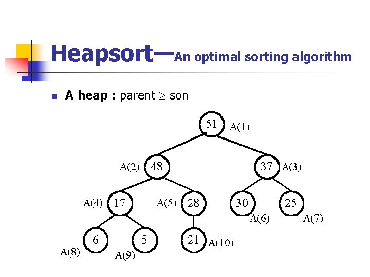
Heapsort—An optimal sorting algorithm n A heap : parent son

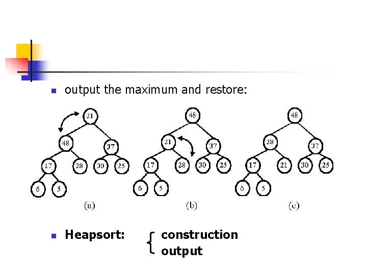
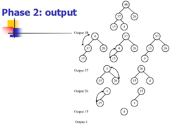
n output the maximum and restore: n Heapsort: construction output

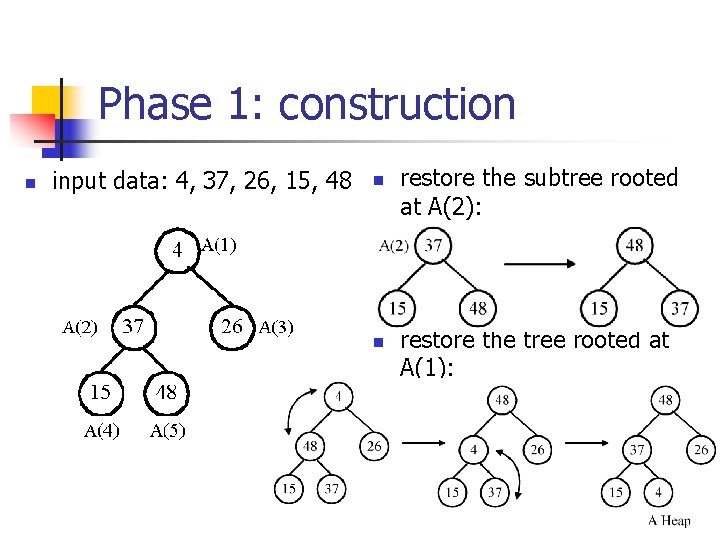
Phase 1: construction n input data: 4, 37, 26, 15, 48 n n restore the subtree rooted at A(2): restore the tree rooted at A(1):

Phase 2: output

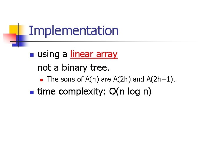
Implementation n using a linear array not a binary tree. n n The sons of A(h) are A(2 h) and A(2 h+1). time complexity: O(n log n)

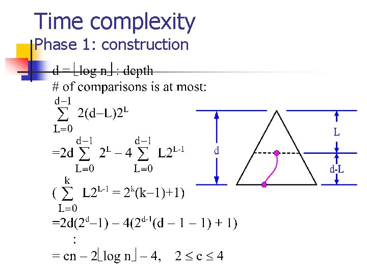
Time complexity Phase 1: construction

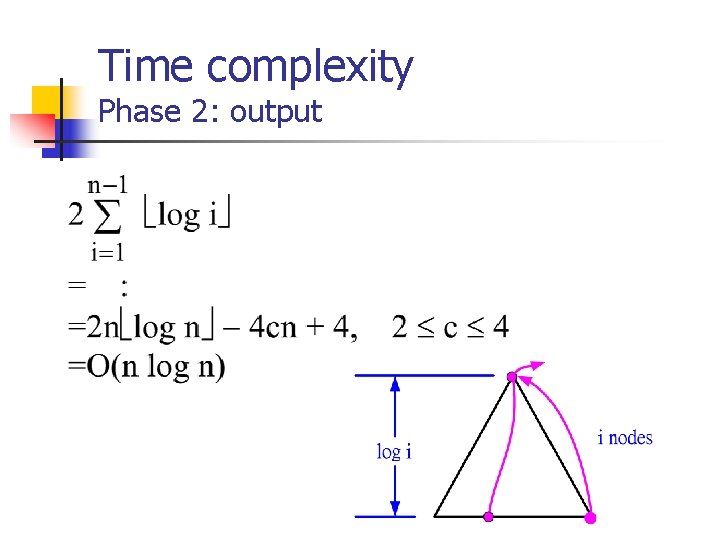
Time complexity Phase 2: output

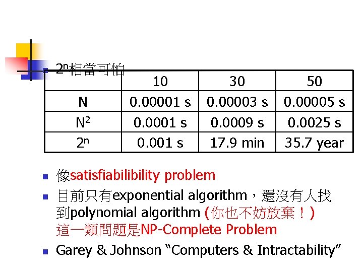
n 2 n相當可怕 N N 2 2 n n 10 0. 00001 s 0. 001 s 30 0. 00003 s 0. 0009 s 17. 9 min 50 0. 00005 s 0. 0025 s 35. 7 year 像satisfiability problem 目前只有exponential algorithm，還沒有人找 到polynomial algorithm (你也不妨放棄！) 這一類問題是NP-Complete Problem Garey & Johnson “Computers & Intractability”

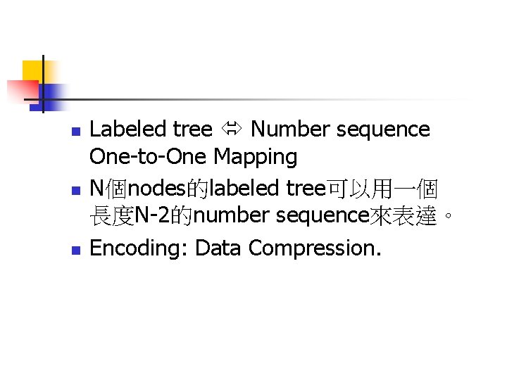
n n n Labeled tree Number sequence One-to-One Mapping N個nodes的labeled tree可以用一個 長度N-2的number sequence來表達。 Encoding: Data Compression.

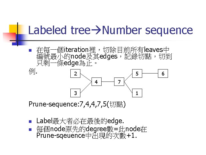
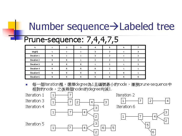
Labeled tree Number sequence 在每一個iteration裡，切除目前所有leaves中 編號最小的node及其edges，記錄切點，切到 只剩一條edge為止。 例. 2 5 6 n 4 7 3 1 Prune-sequence: 7, 4, 4, 7, 5(切點) n n Label最大者必在最後的edge. 每個node原先的degree數=此node在 Prune-sqeuence中出現的次數+1.

Number sequence Labeled tree Prune-sequence: 7, 4, 4, 7, 5 k 1 2 3 4 5 6 7 deg(k) 1 1 1 3 2 1 3 Iteration 1 0 1 1 3 2 1 2 Iteration 2 0 0 1 2 2 1 2 Iteration 3 0 0 0 1 2 Iteration 4 0 0 2 1 1 Iteration 5 0 0 1 0 1 Iteration 6 0 0 0 0 每一個iteration裡，選擇degree為 1且編號最小的node，連接prune-sequence中 相對的node，之後兩個nodes的degree均減 1. 1 7 Iteration 1 Iteration 2 1 7 2 4 Iteration 3 1 7 2 4 3 Iteration 4 Iteration 6 3 n 1 7 3 4 2 Iteration 5 1 7 6 4 2 3 1 7 5 5 6

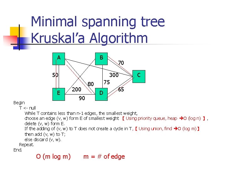
Minimal spanning tree Kruskal’a Algorithm A B 50 E 80 200 90 D 70 300 75 65 C Begin T <- null While T contains less than n-1 edges, the smallest weight, choose an edge (v, w) form E of smallest weight 【 Using priority queue, heap O (log n) 】, delete (v, w) form E. If the adding of (v, w) to T does not create a cycle in T, 【 Using union, find O (log m)】 then add (v, w) to T; else discard (v, w). Repeat. End. O (m log m) m = # of edge

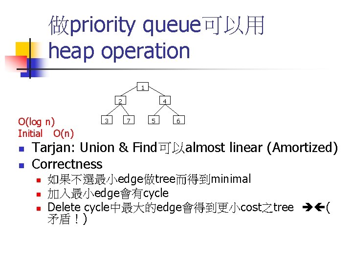
做priority queue可以用 heap operation 1 2 O(log n) Initial O(n) n n 3 4 7 5 6 Tarjan: Union & Find可以almost linear (Amortized) Correctness n n n 如果不選最小edge做tree而得到minimal 加入最小edge會有cycle Delete cycle中最大的edge會得到更小cost之tree ( 矛盾！)

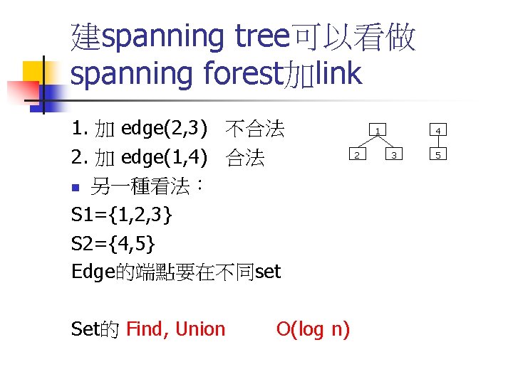
建spanning tree可以看做 spanning forest加link 1. 加 edge(2, 3) 不合法 2. 加 edge(1, 4) 合法 n 另一種看法： S 1={1, 2, 3} S 2={4, 5} Edge的端點要在不同set Set的 Find, Union O(log n) 1 2 4 3 5