Chapter 5 The Structure of TeachT Computer Program

Chapter 5 The Structure of Teach-T Computer Program 5. 1 Purpose and scope of present chapter 1. Purpose: To describe the capabilities, principles of organisation and structure of the TEACH-T program for calculation of 2 -D turbulent recirculating flows. 2. Contents: • Outline of main features of the program. • Details of grid specification, storage of variables, control of iteration, etc. • Description of individual subroutines.

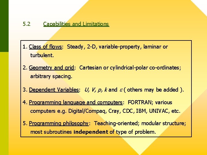
5. 2 Capabilities and Limitations 1. Class of flows: Steady, 2 -D, variable-property, laminar or turbulent. 2. Geometry and grid: Cartesian or cylindrical-polar co-ordinates; arbitrary spacing. 3. Dependent Variables: U, V, p, k and ( others may be added ). 4. Programming language and computers: FORTRAN; various computers e. g. Digital/Compaq, Cray, CDC, IBM, UNIVAC, etc. 5. Programming philosophy: Teaching-oriented; modular structure; most subroutines independent of type of problem.

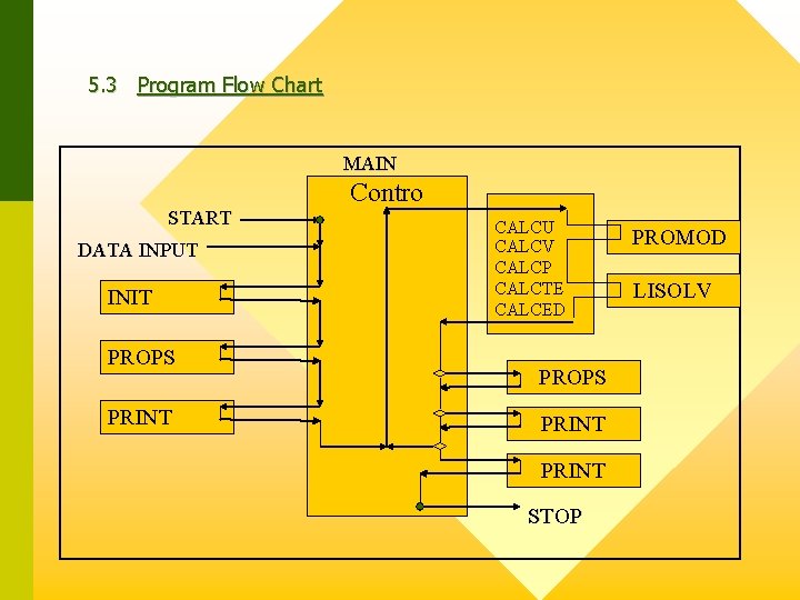
5. 3 Program Flow Chart MAIN START DATA INPUT INIT PROPS PRINT Contro CALCU CALCV CALCP CALCTE CALCED PROPS PRINT STOP PROMOD LISOLV

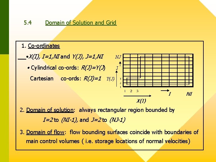
5. 4 Domain of Solution and Grid 1. Co-ordinates • X(I), I=1, NI and Y(J), J=1, NI NJ • Cylindrical co-ords: R(J)=Y(J) J Cartesian co-ords: R(J)=1 Y(J) I NI X(I) 2. Domain of solution: always rectangular region bounded by I=2 to (NI-1), and J=2 to (NJ-1) 3. Domain of flow: flow bounding surfaces coincide with boundaries of main control volumes ( i. e. storage locations of normal velocities)

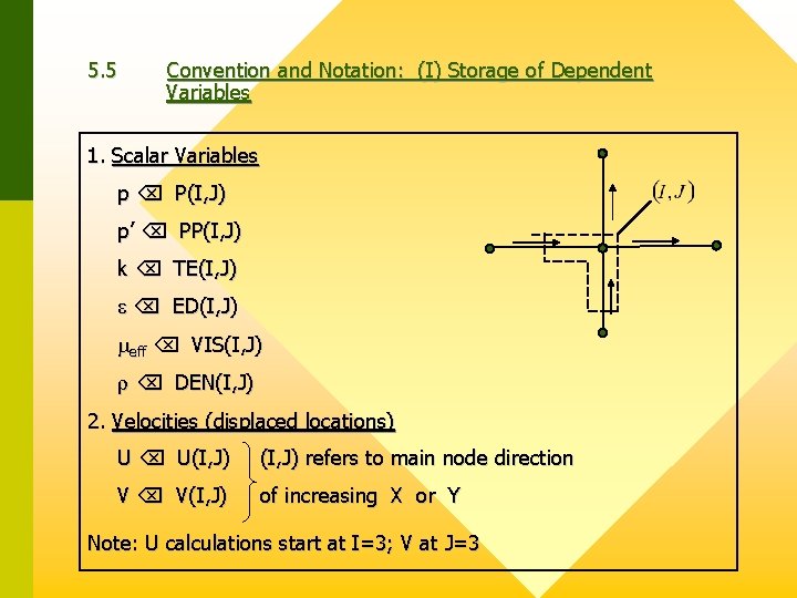
5. 5 Convention and Notation: (I) Storage of Dependent Variables 1. Scalar Variables p P(I, J) p’ PP(I, J) k TE(I, J) ED(I, J) eff VIS(I, J) DEN(I, J) 2. Velocities (displaced locations) U U(I, J) refers to main node direction V V(I, J) of increasing X or Y Note: U calculations start at I=3; V at J=3

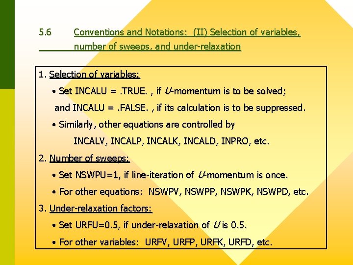
5. 6 Conventions and Notations: (II) Selection of variables, number of sweeps, and under-relaxation 1. Selection of variables: • Set INCALU =. TRUE. , if U-momentum is to be solved; and INCALU =. FALSE. , if its calculation is to be suppressed. • Similarly, other equations are controlled by INCALV, INCALP, INCALK, INCALD, INPRO, etc. 2. Number of sweeps: • Set NSWPU=1, if line-iteration of U-momentum is once. • For other equations: NSWPV, NSWPP, NSWPK, NSWPD, etc. 3. Under-relaxation factors: • Set URFU=0. 5, if under-relaxation of U is 0. 5. • For other variables: URFV, URFP, URFK, URFD, etc.

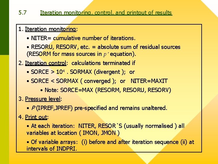
5. 7 Iteration monitoring, control, and printout of results 1. Iteration monitoring: • NITER= cumulative number of iterations. • RESORU, RESORV, etc. = absolute sum of residual sources (RESORM for mass sources in p’ equation). 2. Iteration control: calculations terminated if • SORCE > 104. SORMAX (divergent ); or • SORCE < SORMAX ( converged ); or NITER=MAXIT • Note: SORCE=MAX (RESORM, RESORU, RESORV) 3. Pressure level: • P (IPREF, JPREF) pre-specified and remains unaltered. 4. Print out: • At each iteration: NITER, RESOR´S (usually normalised ) all variables at location ( IMON, JMON ) • Of variable arrays: (i) before and after iteration sequence (ii) at intervals of INDPRI.

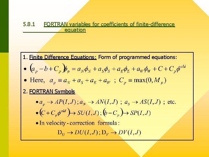
5. 8. 1 FORTRAN variables for coefficients of finite-difference equation 1. Finite Difference Equations; Form of programmed equations: 2. FORTRAN Symbols

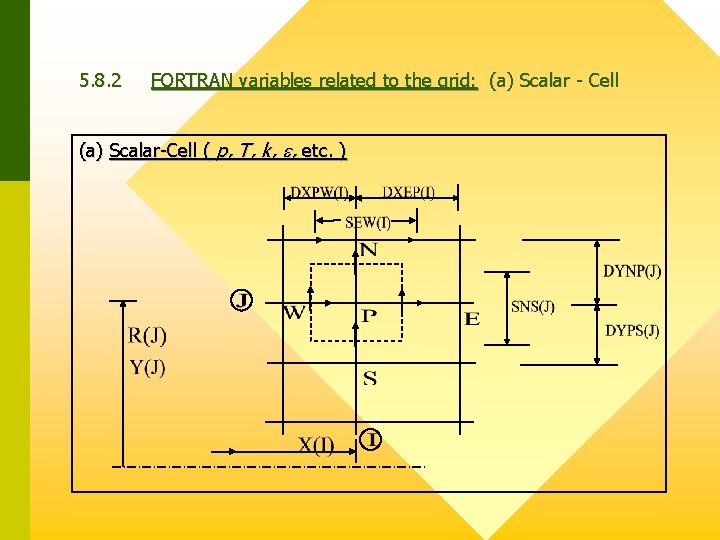
5. 8. 2 FORTRAN variables related to the grid: (a) Scalar - Cell (a) Scalar-Cell ( p, T, k, , etc. )

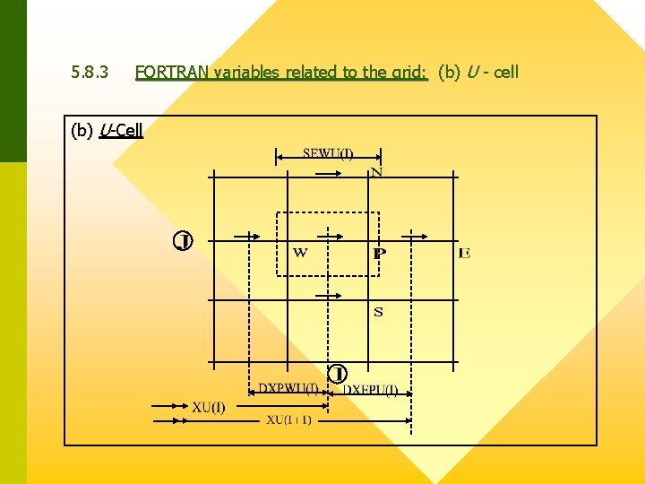
5. 8. 3 FORTRAN variables related to the grid: (b) U - cell (b) U-Cell

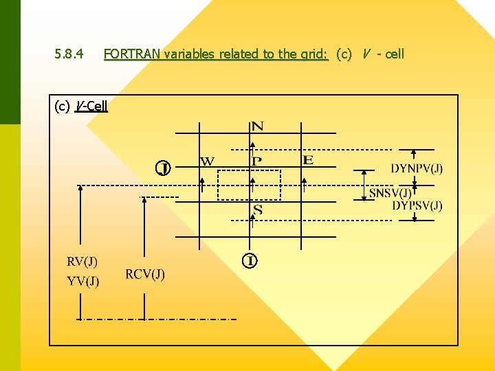
5. 8. 4 FORTRAN variables related to the grid: (c) V - cell (c) V-Cell

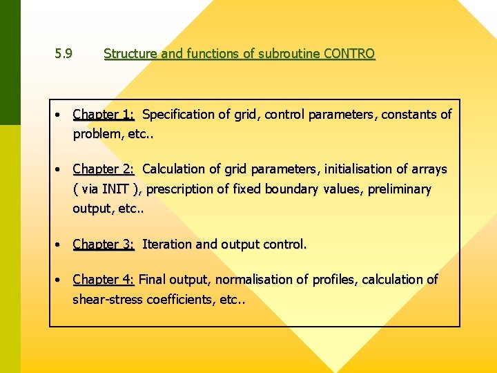
5. 9 Structure and functions of subroutine CONTRO • Chapter 1: Specification of grid, control parameters, constants of problem, etc. . • Chapter 2: Calculation of grid parameters, initialisation of arrays ( via INIT ), prescription of fixed boundary values, preliminary output, etc. . • Chapter 3: Iteration and output control. • Chapter 4: Final output, normalisation of profiles, calculation of shear-stress coefficients, etc. .

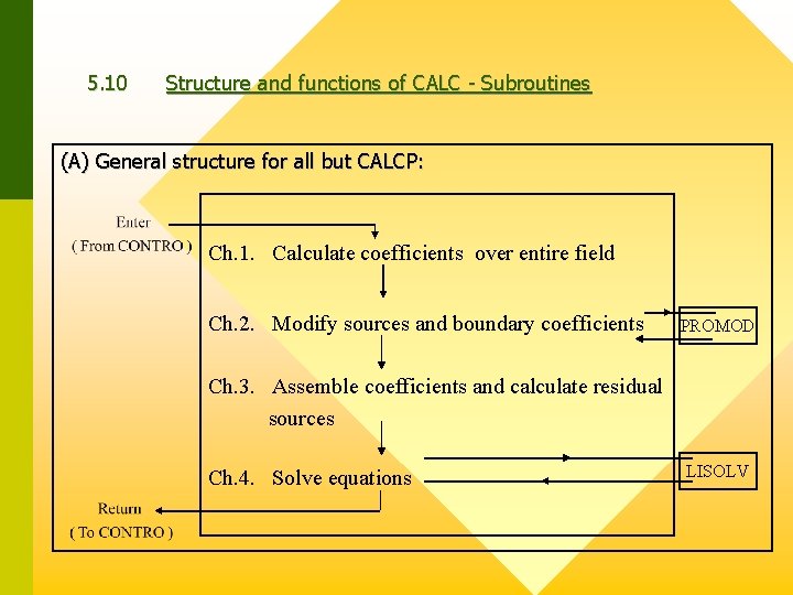
5. 10 Structure and functions of CALC - Subroutines (A) General structure for all but CALCP: Ch. 1. Calculate coefficients over entire field Ch. 2. Modify sources and boundary coefficients PROMOD Ch. 3. Assemble coefficients and calculate residual sources Ch. 4. Solve equations LISOLV

5. 11 Structure and function of CALC - Subroutines ( cont’d) (B) Special features of CALCP: 1. an’s are unlikely all to become zero: so no special precautions are taken. 2. In Ch. 1 absolute mass sources are summed and stored as as RESORM. 3. Residual source of p’ equation provide no useful information, so they are not calculated. 4. Corrections are applied to pressures and velocities in (additional) chapter 5.

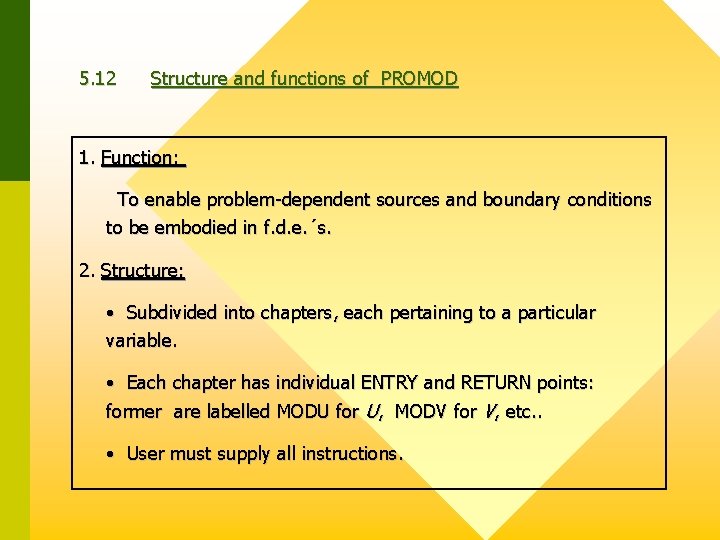
5. 12 Structure and functions of PROMOD 1. Function: To enable problem-dependent sources and boundary conditions to be embodied in f. d. e. ´s. 2. Structure: • Subdivided into chapters, each pertaining to a particular variable. • Each chapter has individual ENTRY and RETURN points: former are labelled MODU for U, MODV for V, etc. . • User must supply all instructions.

5. 13 Structure and function of PROPS and LISOLV 1. PROPS: Calculates values over entire field of thermodynamic and transport properties ( e. g. , eff , etc. ). 2. LISOLV: Applies line-iteration algorithm, arranged to solve along N-S lines, with W-E sweeps. Important arguments are: PHI(I, J) - array containing variable to be computed ISTART, JSTART- starting indices of traverses and sweeps.

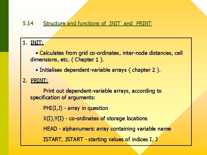
5. 14 Structure and functions of INIT and PRINT 1. INIT: • Calculates from grid co-ordinates, inter-node distances, cell dimensions, etc. ( Chapter 1 ). • Initialises dependent-variable arrays ( chapter 2 ). 2. PRINT: Print out dependent-variable arrays, according to specification of arguments: PHI(I, J) - array in question X(I), Y(I) - co-ordinates of storage locations HEAD - alphanumeric array containing variable name ISTART, JSTART - starting values of indices I, J

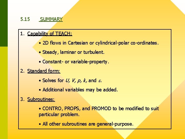
5. 15 SUMMARY 1. Capability of TEACH: • 2 D flows in Cartesian or cylindrical-polar co-ordinates. • Steady, laminar or turbulent. • Constant- or variable-property. 2. Standard form: • Solves for U, V, p, k, and . • Additional variables may be added. 3. Subroutines: • CONTRO, PROPS, and PROMOD to be modified to suit particular problem. • All other subroutines are general-purpose.