CHAPTER 5 THE DISCRETETIME FOURIER TRANSFORM 5 0

CHAPTER 5 THE DISCRETE-TIME FOURIER TRANSFORM 5. 0 INTRODUCTION • Discrete-time Fourier transform and inverse Fourier transform. • Similarities and differences between continuous-time and discrete-time Fourier transforms.

5. 1 REPRESENTATION OF APERIODIC SIGNALS: THE DISCRETE-TIME FOURIER TRANSFORM … … –N –N 1 0 N 2 n N x[n] As , –N 1 0 N 2 n

Defining a function: Thus, Consequently, As discrete-time Fourier transform , discrete-time inverse Fourier transform

ØDifferences between the continuous-time and discrete-time Fourier transform are: periodicity of the discrete-time transform and the finite interval of integration in the synthesis equation. x 1[n] 0 – 2π–π 0 π 2π x 2[n] n 0 ω n – 2π –π 0 π 2π ØIn discrete time, Low frequencies are the values of ω near even multiple of π ; high frequencies are those values of ω near odd multiples of π. ω

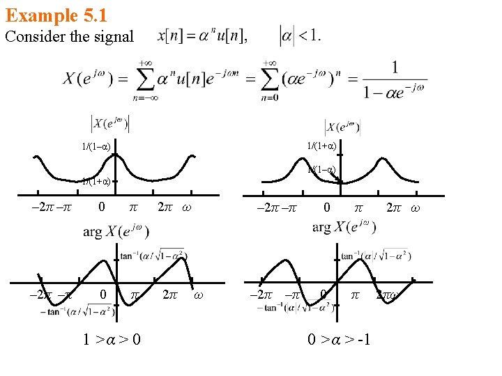
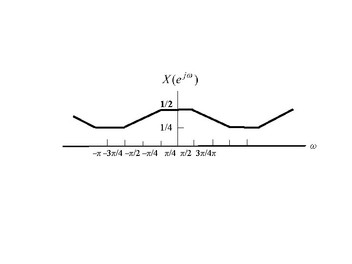
Example 5. 2 Consider the signal for 0 < α < 1, x[n] (1+α)/(1–α)/(1+α) 0 n – 2π 0 2π ω

Example 5. 3 Consider the rectangular pulse x[n] 1 –N 10 N 1 5 – 2π –π 0 π 2π ω n

ØConvergence Issues of the Discrete-Time Fourier Transform • If x[n] is an infinite duration signal, we must consider the question of convergence of the infinite summation in the analysis equation. • The analysis equation will converge if x[n] is absolutely summable; that is • In contrast to the situation for the analysis equation, there are generally no convergence issues associated with the synthesis equation.

Approximation to the unit sample obtained as in eq. (5. 13) using complex exponentials with frequencies |ω| ≤ W: (a) W = π/4; (b) W = 3π/8; (c) W = π/2; (d) W = 3π/4; (e) W = 7π/8; (f) W = π. Note that for W = π,

5. 2 THE FOURIER TRANSFORM FOR PERIODIC SIGNALS First consider the Fourier transform of the sequence 2π … … To check the validity of this expression, ω (ω0– 4π) ω0 (ω0– 2π) (ω0+4π) (ω0+2π)

Now consider an arbitrary periodic sequence x[n] with period N and with the Fourier series representation. Applying the Fourier transform to both sides, we obtain Thus, the Fourier transform of a periodic signal can be directly constructed from its Fourier coefficients. Example 5. 4 Consider the periodic signal

That is, π … … – 2π –ω0 0 ω0 2π (– 2π–ω0) (– 2π+ω0) (2π–ω0) (2π+ω0) Example 5. 5 Consider the periodic sample train x[n] 1 … –N 0 N … 2 N n ω

Choosing the interval of summation as 0 ≤ n ≤ N-1, Then we can represent the Fourier transform of the signal as 2π/N … … ω

5. 3 PROPERTIES OF THE DISCRETE-TIME FOURIER TRANSFORM 5. 3. 1 Periodicity of the Discrete-Time Fourier Transform 5. 3. 2 Linearity of the Fourier Transform If and then 5. 3. 3 Time Shifting and Frequency Shifting If then and

5. 3. 4 Conjugation and Conjugate Symmetry If then if x[n] is real valued,

5. 3. 5 Differencing and Accumulation First-difference: Accumulation: 5. 3. 6 Time Reversal 5. 3. 7 Time Expansion If then

5. 3. 8 Differentiation in Frequency 5. 3. 9 Parseval’s Relation

Example 5. 6 The frequency response of a discrete-time low-pass filter with cutoff frequency ωc is illustrated in the next figure: 1 – 2π If we shift –π –(π–ωc) ωc π 2π ω by one-half period, i. e. , by π, then we obtain: 1 – 2π –π –ωc π (π–ωc) 2π ω

Example 5. 7 Consider the unit step sequence u[n]. Since and Thus,

Example 5. 8 Consider the sequence x[n] which is illustrated in the following figure: 2 x[n] 1 y[n] 1 0 1 2 3 4 5 6 7 8 9 n y(2)[n] 1 0 1 2 3 4 5 6 7 8 9 n 2 2 y(2)[n-1] 0 1 2 3 4 5 6 7 8 9 n n

5. 4 THE CONVOLUTION PROPERTY If then ØThe convolution property represents that the Fourier transform of the response of an LTI system to a nonperiodic input are simply the Fourier transform of the input multiplied by the system’s frequency response evaluated at the corresponding frequencies. ØThe convolution property maps the convolution operation of two time signals to the multiplication operation of their Fourier transforms. ØThe frequency response captures the change in complex amplitude of the Fourier transform of the input at each frequency ω.

Example 5. 8 Consider an LTI system with sample response The frequency response is Thus, for any input x[n], the Fourier transform of the output is Consequently, Magnitude = 1 at all frequencies phase =

Example 5. 9 Consider an LTI system with sample response The input to this system is The output y[n] = ? If

Thus, If

Example 5. 10 w 1[n] Consider the system w 2[n] x[n] w 3[n] + w 4[n] y[n] What is the frequency response of the overall system? Where is an ideal low-pass filter with cutoff frequency π/4 and unity gain in the passband. The key procedure: Thus, Since,

Consequently, From the convolution property, the overall system has the frequency response: ideal bandstop filter 1 ω –π – 3π/4 –π/4 3π/4 π Stopband:

5. 5 THE MULTIPLICATION PROPERTY Consider the Fourier transform of y[n] = x 1[n] x 2[n], where the Fourier transforms of x 1[n] and x 2[n] are known. since periodic convolution

Example 5. 11 Consider the problem of finding the Fourier transform signal x[n] which is the product of x 1[n] and x 2[n], where 1 1 ω – 2π –π –π/2 π of a 2π From the multiplication property, – 2π –π– 3π/4π 2π ω

5. 6 DUALITY SUMMARY OF FOURIER SERIES AND TRANSFORM EXPRESSIONS Continuous time Fourier Series Discrete time Time domain Frequency domain Time domain continuous time periodic in time discrete frequency aperiodic in frequency Frequency domain duality discrete frequency periodic in frequency du ali ty Fourier Transform continuous frequency continuous time aperiodic in timeduality aperiodic in frequency discrete time aperiodic in time continuous frequency periodic in frequency

ØFor the discrete-time Fourier series, duality between the sequence x[n] in the time-domain and its Fourier series coefficient f [k] is: ØFor the continuous-time Fourier transform, duality between the signal x(t) in the time-domain and its Fourier transform X(jω) is: ØDuality implies that every property has a dual. ØThere is also a duality between the discrete-time Fourier transform and the continuous-time Fourier series. the nth Fourier coefficient is x[–n] is periodic, and all of its harmonically related components have the common period of 2π synthesis equation analysis equation

Example 5. 12 Determine the discrete-time Fourier transform of the sequence Since the Fourier transform of x[n] is periodic with period 2π, and with the form of square wave, so we consider signal g(t), which is a periodic square wave with period 2π, and with the Fourier series coefficients of g(t) are Let T 1 = π/2, then we have ak = x[k], taking ak and g(t) into the analysis equation:

Renaming k as n and t as ω, we have Replacing n by –n , we obtain Thus,

5. 7 SYSTEMS CHARACTERIZED BY LINEAR CONSTANT-COEFFICIENT DIFFERENCE EQUATIONS is a ratio of polynomials in the variable. Øcoefficients of the numerator polynomial = coefficients appearing on the right side of the difference equation. Øcoefficients of the denominator polynomial = coefficients appearing on the left side of the difference equation. Ø

Example 5. 13 Consider a causal LTI system that is characterized by the difference equations and let the input to this system be Determine the output y[n]. The form of the partial-fraction expansion in this case is

So that, Consequently,

5. 8 DISCRETE-TIME FREQUENCY-SELECTIVE FILTER ideal low-pass filter 1 – 2π –π –ωc 0 ωc ω 2π π ω 2π 1 ideal high-pass filter –π ideal band-pass filter – 2π –π π ideal band-stop filter π 2π ω ω

5. 9 SAMPLING OF DISCRETE-TIME SIGNALS x[n] Χ xp[n] x[n] n p[n] n xp[n] n Impulse-train sampling

spectrum of original signal 1 ω – 2π spectrum of sampling sequence –ωM ωM 2π 2π/N ωs spectrum of sampled signal with ωs > 2ωM spectrum of sampled signal with ωs < 2ωM 2π ω 1/N –ωM ωM ωs (ωs – ωM) 2π ω 1/N ωs 2π In discrete-time case, the result of sampling theorem also exist. ω

Example 5. 14 Consider a sequence x[n] whose Fourier transform Determine the lowest rate at which x[n] may be sampled without aliasing. Since From the sampling theorem, we know So that Thus the corresponding sampling frequency is 2π/4 = π/2.

5. 10 SUMMARY ØThe Fourier transform for aperiodic discrete-time signals; ØThe Fourier transform for periodic discrete-time signals; ØThe difference between the continuous-time Fourier transform and the discrete-time Fourier transform (the discrete-time Fourier transform of an aperiodic signal is always periodic with period 2π); ØThe properties of the Fourier transform (how different characteristics of signals are reflected in their transforms); ØFourier analysis method (also referred to frequency-domain analysis)(which is to used to change a linear constant-coefficient difference equation to an algebraic form); ØConvenient way to obtain the frequency response and sample response of a discrete-time LTI system; ØSampling of discrete-time signals.