Chapter 5 Section 5 1 Statistics MR ZBORIL

Chapter 5 Section 5. 1 Statistics MR. ZBORIL | MILFORD PEP This Photo by Unknown Author is licensed under CC BY-NCND

Chapter 5 Section 5. 1 Intro to Random Variables You are important to me – don’t ever think otherwise! This Photo y Unknown Author is licensed under CC BY-SA

Section 5. 1 Introduction to Random Variations and Probability Distributions Focus Points • Distinguish between discrete and continuous random variables. • Graph discrete probability distributions • Compute μ and σ for a discrete probability distributions. • Compute μ and σ for a linear function of a random variable x. • Compute μ and σ for a linear combination of two independent random variables.

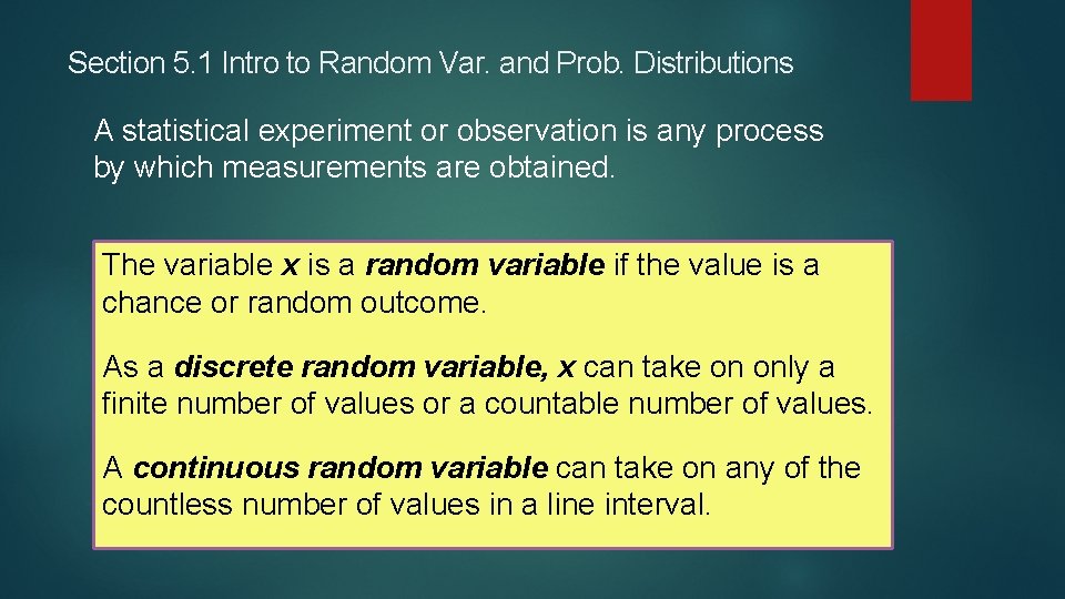
Section 5. 1 Intro to Random Var. and Prob. Distributions A statistical experiment or observation is any process by which measurements are obtained. The variable x is a random variable if the value is a chance or random outcome. As a discrete random variable, x can take on only a finite number of values or a countable number of values. A continuous random variable can take on any of the countless number of values in a line interval.

Section 5. 1 Intro to Random Var. and Prob. Distributions Guided Exercise 1 Determine which of the following are discrete and which are continuous. Count usually indicates a discrete random variable. Measure usually indicates a continuous random variable.

Section 5. 1 Intro to Random Var. and Prob. Distributions Look at Example 1 at the bottom of page 183. This is an example of what is called a probability distribution. Dr. Mendoza created a Boredom Tolerance Test. This is used to determine if a job applicant would be a good fit for reperforming a repeated, monotonous task. The 0, 1, 2, 3, 4, 5, 6 possible scores are an example of a discrete random variable. The test results are shown in Figure 5 -1 and the Probability Distribution is shown in Figure 5 -2.

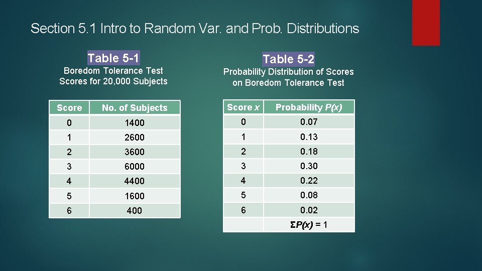
Section 5. 1 Intro to Random Var. and Prob. Distributions Table 5 -1 Boredom Tolerance Test Scores for 20, 000 Subjects Table 5 -2 Probability Distribution of Scores on Boredom Tolerance Test Score No. of Subjects Score x Probability P(x) 0 1400 0 0. 07 1 2600 1 0. 13 2 3600 2 0. 18 3 6000 3 0. 30 4 4400 4 0. 22 5 1600 5 0. 08 6 400 6 0. 02 ΣP(x) = 1

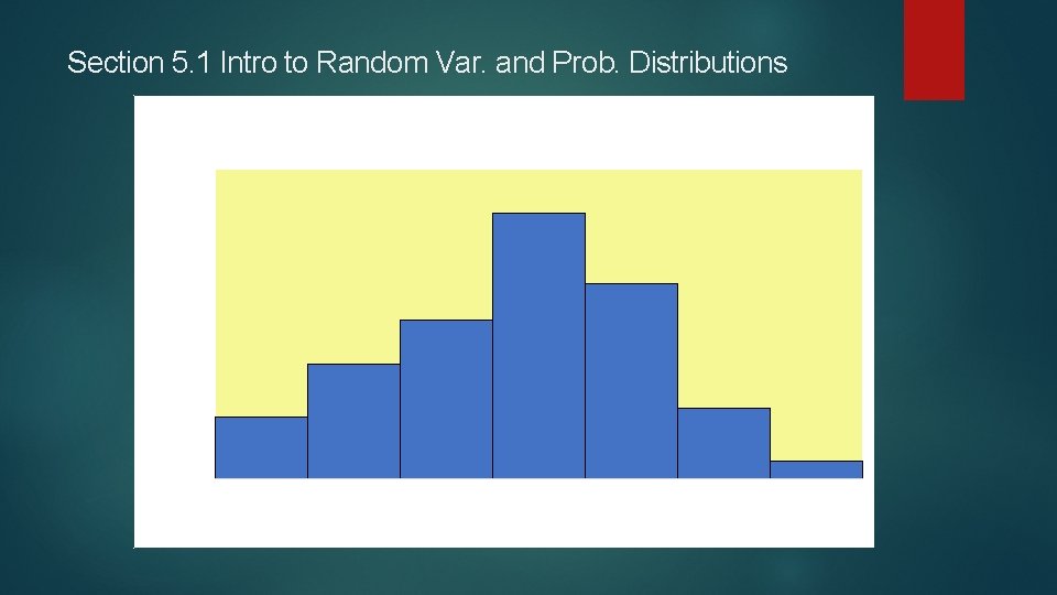
Section 5. 1 Intro to Random Var. and Prob. Distributions FIGURE 5 -1 Graph of the Probability Distribution of Test Scores 0, 35 0, 3 Probability P(x) 0, 25 0, 2 0, 15 0, 1 0, 05 0 0 1 2 3 Boredom Scores x 4 5 6

Section 5. 1 Intro to Random Var. and Prob. Distributions A probability distribution can be thought of as a relative-frequency distribution based on a very large n. It has both a mean and standard deviation. In Chapter 3 we learned how to calculate the mean for a series of raw data. We also learned how to calculate the standard deviation. Chapter 5 is different!! Now our old friends are returning and being applied to probability distributions. Calculating sums is fun! I’m back! We’re your forever friends!

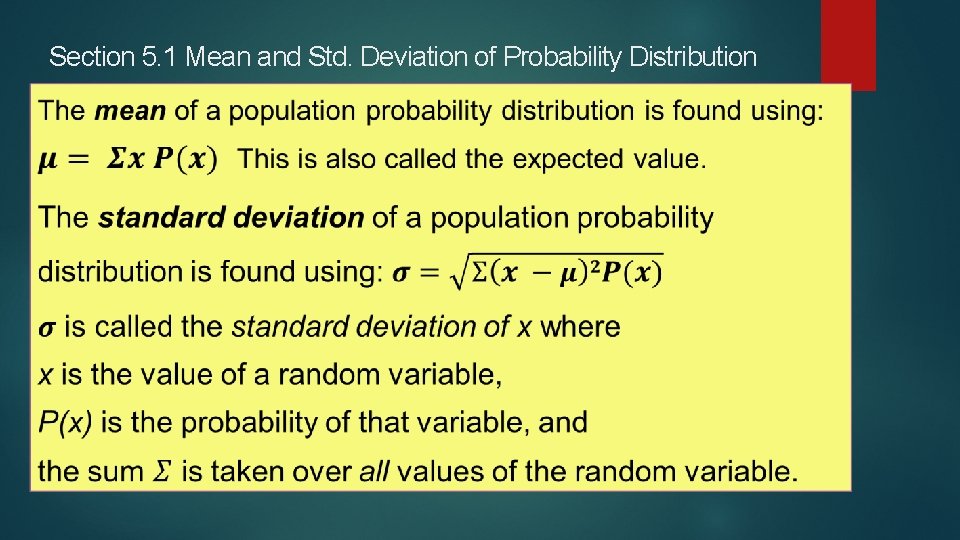
Section 5. 1 Mean and Std. Deviation of Probability Distribution

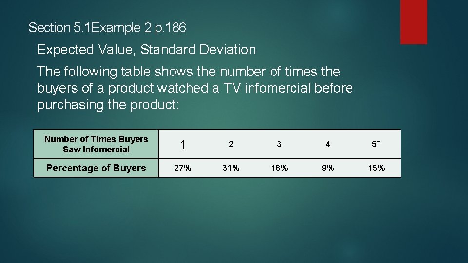
Section 5. 1 Example 2 p. 186 Expected Value, Standard Deviation The following table shows the number of times the buyers of a product watched a TV infomercial before purchasing the product: Number of Times Buyers Saw Infomercial 1 2 3 4 5* Percentage of Buyers 27% 31% 18% 9% 15%

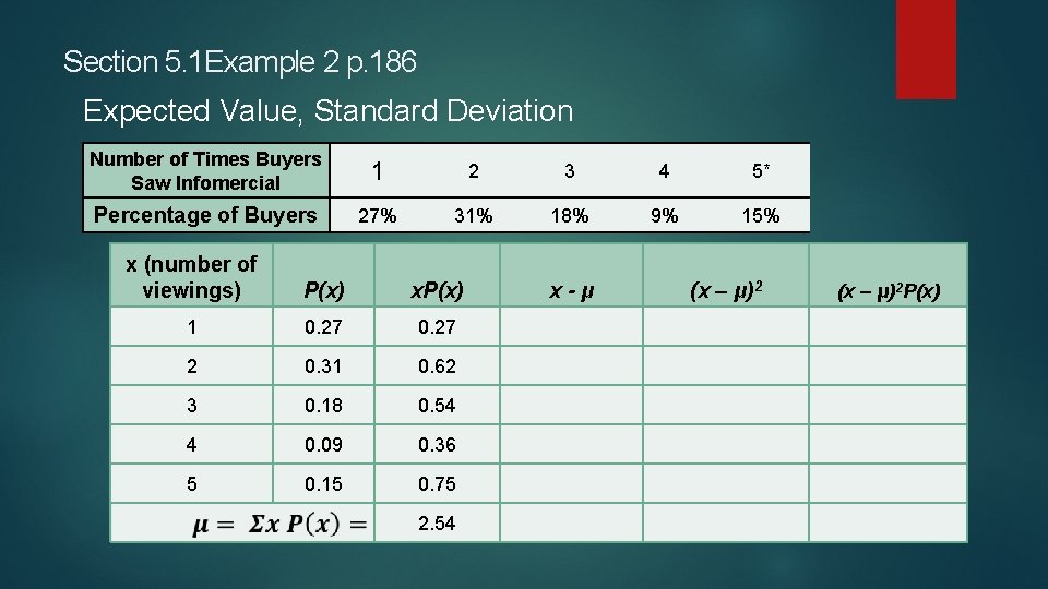
Section 5. 1 Example 2 p. 186 Expected Value, Standard Deviation Number of Times Buyers Saw Infomercial 1 2 3 4 5* Percentage of Buyers 27% 31% 18% 9% 15% x (number of viewings) P(x) x. P(x) 1 0. 27 2 0. 31 0. 62 3 0. 18 0. 54 4 0. 09 0. 36 5 0. 15 0. 75 2. 54 x-μ (x – μ)2 P(x)

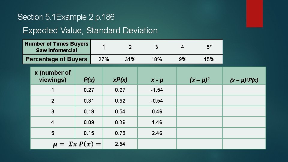
Section 5. 1 Example 2 p. 186 Expected Value, Standard Deviation Number of Times Buyers Saw Infomercial 1 2 3 4 5* Percentage of Buyers 27% 31% 18% 9% 15% x (number of viewings) P(x) x-μ 1 0. 27 -1. 54 2 0. 31 0. 62 -0. 54 3 0. 18 0. 54 0. 46 4 0. 09 0. 36 1. 46 5 0. 15 0. 75 2. 46 2. 54 (x – μ)2 P(x)

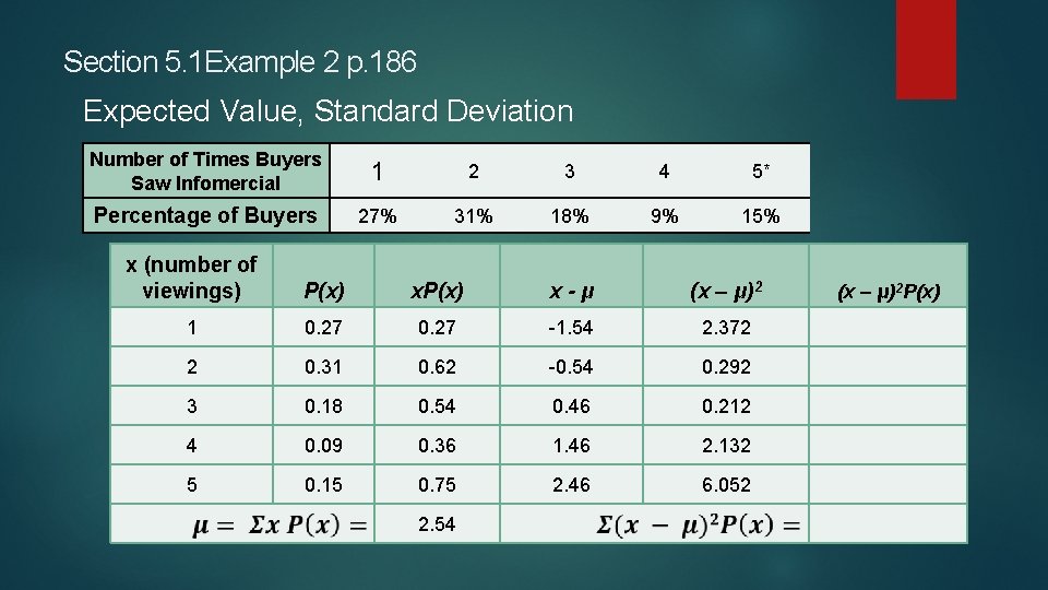
Section 5. 1 Example 2 p. 186 Expected Value, Standard Deviation Number of Times Buyers Saw Infomercial 1 2 3 4 5* Percentage of Buyers 27% 31% 18% 9% 15% x (number of viewings) P(x) x-μ (x – μ)2 1 0. 27 -1. 54 2. 372 2 0. 31 0. 62 -0. 54 0. 292 3 0. 18 0. 54 0. 46 0. 212 4 0. 09 0. 36 1. 46 2. 132 5 0. 15 0. 75 2. 46 6. 052 2. 54 (x – μ)2 P(x)

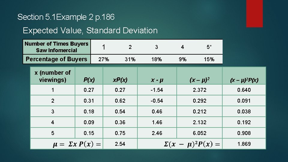
Section 5. 1 Example 2 p. 186 Expected Value, Standard Deviation Number of Times Buyers Saw Infomercial 1 2 3 4 5* Percentage of Buyers 27% 31% 18% 9% 15% x (number of viewings) P(x) x-μ (x – μ)2 P(x) 1 0. 27 -1. 54 2. 372 0. 640 2 0. 31 0. 62 -0. 54 0. 292 0. 091 3 0. 18 0. 54 0. 46 0. 212 0. 038 4 0. 09 0. 36 1. 46 2. 132 0. 192 5 0. 15 0. 75 2. 46 6. 052 0. 908 2. 54 1. 869

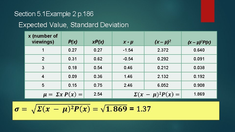
Section 5. 1 Example 2 p. 186 Expected Value, Standard Deviation x (number of viewings) P(x) x-μ (x – μ)2 P(x) 1 0. 27 -1. 54 2. 372 0. 640 2 0. 31 0. 62 -0. 54 0. 292 0. 091 3 0. 18 0. 54 0. 46 0. 212 0. 038 4 0. 09 0. 36 1. 46 2. 132 0. 192 5 0. 15 0. 75 2. 46 6. 052 0. 908 2. 54 1. 869

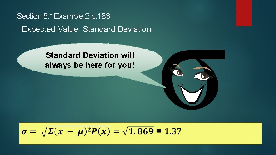
Section 5. 1 Example 2 p. 186 Expected Value, Standard Deviation will always be here for you!

Section 5. 1 Linear Functions of a Random Variable Let a and b be any constant, and let x be a random variable. The new random variable L = a + bx is called a linear function of x.

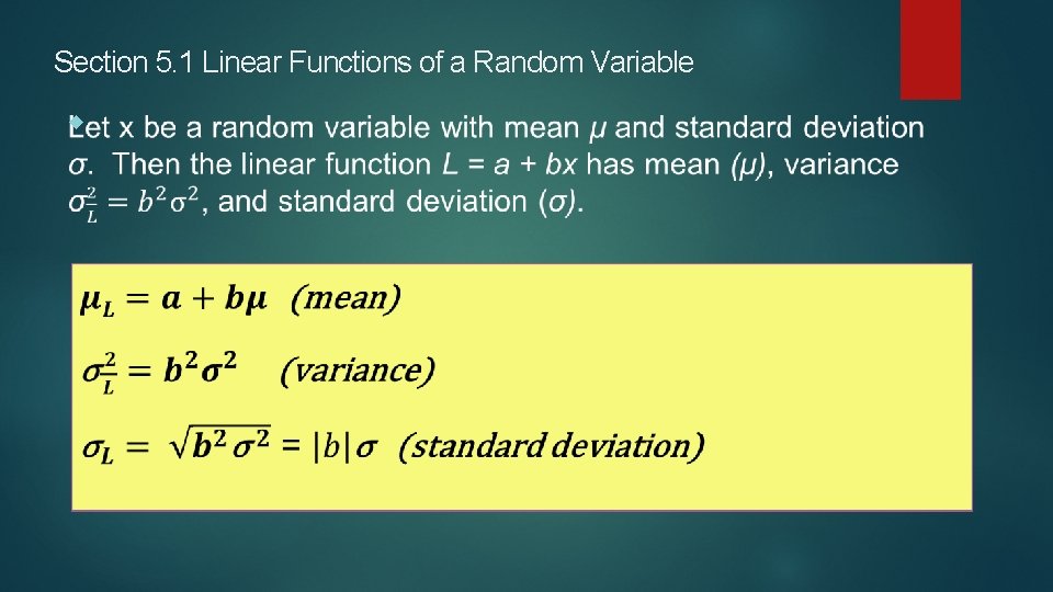
Section 5. 1 Linear Functions of a Random Variable

Section 5. 1 Linear Functions of a Random Variable Let x 1 and x 2 be two independent random variables and a and b be any constants. Then the new random variable W = ax 1 + bx 2 is called a linear combination of x 1 and x 2.

Chapter 5 Section 5. 2 Statistics MR. ZBORIL | MILFORD PEP

Chapter 5 Section 5. 2 Intro to Random Variables Your are important to me – don’t ever think otherwise! This Photo y Unknown Author is licensed under CC BY-SA

Section 5. 2 Binomial Probabilities Focus Points • List the defining features of a binomial experiment. • Compute binomial probabilities using the formula P(r) = C n, r p r q n-r. • Use the binomial table to find P(r). • Use the binomial probability distribution to solve realworld applications.

Section 5. 2 Binomial Probabilities On a game show, contestants are given a spin on the wheel of fortune. The wheel consists of 36 slots – one of which is gold. The gold slot pays $50, 000. No other slot pays. What is the possibility the show will pay $50, 000 to three contestants out of 100?

Section 5. 2 Binomial Probabilities This problem is called a binomial, or Bernoulli experiment. § There are two possible outcomes for each trial – the ball lands on the gold slot, or it does not. § Named after Swiss mathematician Jacob Bernoulli.

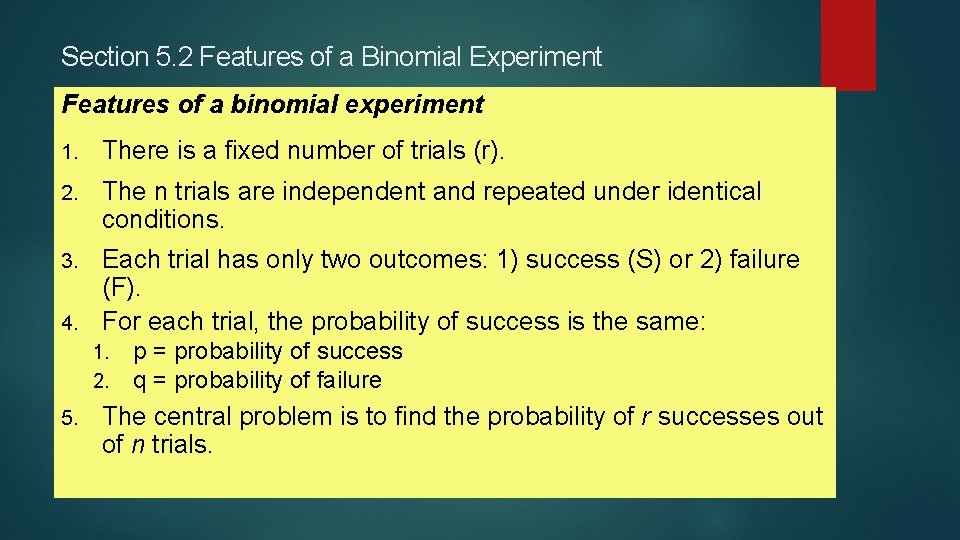
Section 5. 2 Features of a Binomial Experiment Features of a binomial experiment 1. There is a fixed number of trials (r). 2. The n trials are independent and repeated under identical conditions. Each trial has only two outcomes: 1) success (S) or 2) failure (F). 4. For each trial, the probability of success is the same: 3. 1. 2. 5. p = probability of success q = probability of failure The central problem is to find the probability of r successes out of n trials.

Section 5. 2 Binomial Probabilities Example 4 pg. 195 Review the wheel of fortune game against the criteria for a binomial experiment.

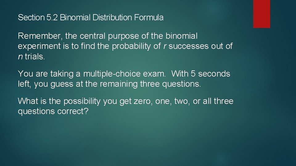
Section 5. 2 Binomial Distribution Formula Remember, the central purpose of the binomial experiment is to find the probability of r successes out of n trials. You are taking a multiple-choice exam. With 5 seconds left, you guess at the remaining three questions. What is the possibility you get zero, one, two, or all three questions correct?

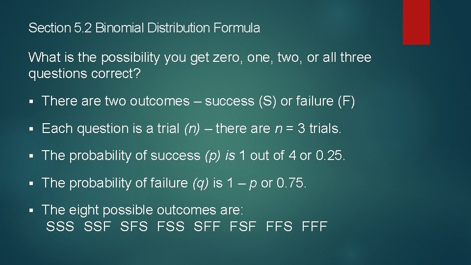
Section 5. 2 Binomial Distribution Formula What is the possibility you get zero, one, two, or all three questions correct? § There are two outcomes – success (S) or failure (F) § Each question is a trial (n) – there are n = 3 trials. § The probability of success (p) is 1 out of 4 or 0. 25. § The probability of failure (q) is 1 – p or 0. 75. § The eight possible outcomes are: SSS SSF SFS FSS SFF FSF FFS FFF

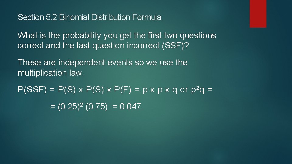
Section 5. 2 Binomial Distribution Formula What is the probability you get the first two questions correct and the last question incorrect (SSF)? These are independent events so we use the multiplication law. P(SSF) = P(S) x P(F) = p x q or p 2 q = = (0. 25)2 (0. 75) = 0. 047.

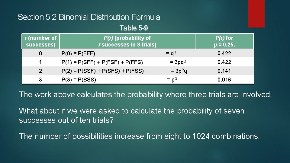
Section 5. 2 Binomial Distribution Formula Table 5 -9 r (number of successes) P(r) (probability of r successes in 3 trials) P(r) for p = 0. 25. 0 P(0) = P(FFF) = q 3 1 P(1) = P(SFF) + P(FSF) + P(FFS) = 3 pq 2 0. 422 2 P(2) = P(SSF) + P(SFS) + P(FSS) = 3 p 2 q 0. 141 3 P(3) = P(SSS) = p 3 0. 422 0. 016 The work above calculates the probability where three trials are involved. What about if we were asked to calculate the probability of seven successes out of ten trials? The number of possibilities increase from eight to 1024 combinations.

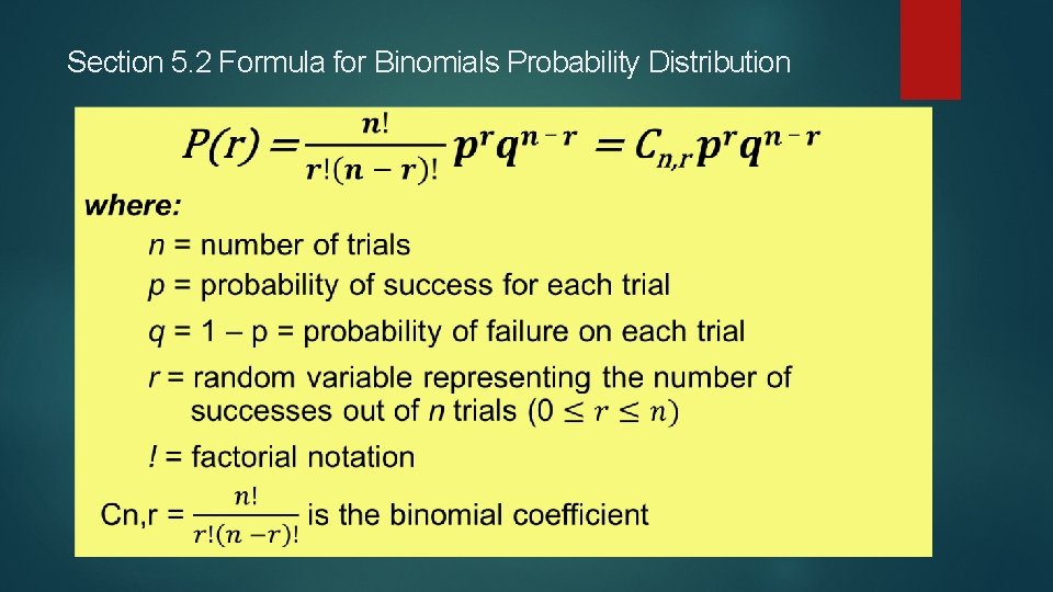
Section 5. 2 Formula for Binomials Probability Distribution

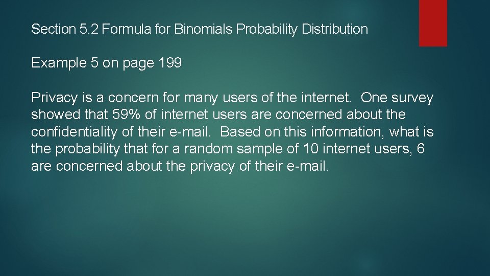
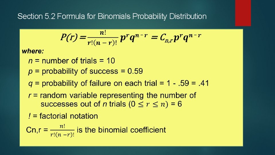
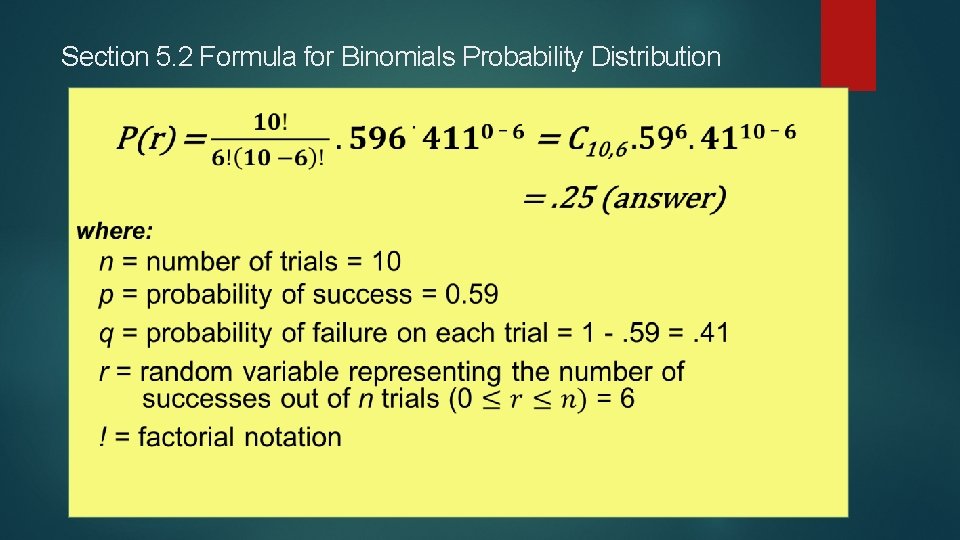
Section 5. 2 Formula for Binomials Probability Distribution Example 5 on page 199 Privacy is a concern for many users of the internet. One survey showed that 59% of internet users are concerned about the confidentiality of their e-mail. Based on this information, what is the probability that for a random sample of 10 internet users, 6 are concerned about the privacy of their e-mail.

Section 5. 2 Formula for Binomials Probability Distribution

Section 5. 2 Formula for Binomials Probability Distribution

Section 5. 2 Binomial Probabilities Questions? This Photo by Unknown Author is licensed under CC BY-SA