Chapter 5 Probability Distributions and Data Modeling Business

Chapter 5: Probability Distributions and Data Modeling Business Analytics: Methods, Models, and Decisions, 1 st edition James R. Evans Copyright © 2013 Pearson Education, Inc. publishing as Prentice Hall 5 -1

Copyright © 2013 Pearson Education, Inc. publishing as Prentice Hall 5 -2

Chapter 5 Topics Basic Concepts of Probability Random Variables and Probability Distributions Discrete Probability Distributions Continuous Probability Distributions Random Sampling from Probability Distributions Data Modeling and Distribution Fitting Copyright © 2013 Pearson Education, Inc. publishing as Prentice Hall 5 -3

Basic Concepts of Probability Probability is the likelihood that an outcome occurs. An experiment is the process that results in an outcome. The outcome of an experiment is a result that we observe. The sample space is the collection of all possible outcomes of an experiment. An event is a collection of one or more outcomes from a sample space. Copyright © 2013 Pearson Education, Inc. publishing as Prentice Hall 5 -4

Basic Concepts of Probability Probabilities may be defined from one of three perspectives: � Classical definition: probabilities can be deduced from theoretical arguments � Relative frequency definition: probabilities are based on empirical data � Subjective definition: probabilities are based on judgment and experience Copyright © 2013 Pearson Education, Inc. publishing as Prentice Hall 5 -5

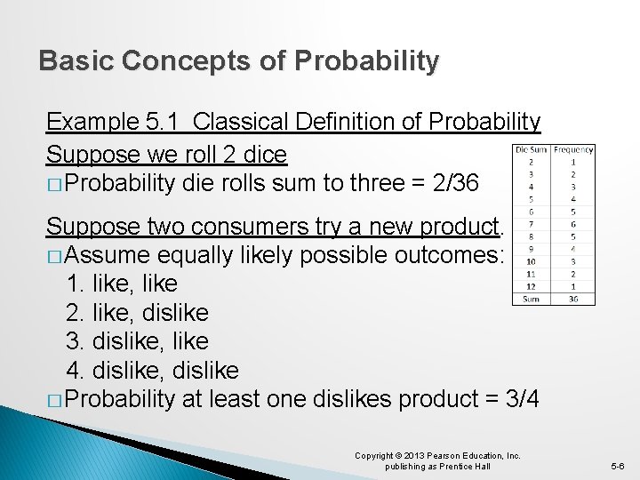
Basic Concepts of Probability Example 5. 1 Classical Definition of Probability Suppose we roll 2 dice � Probability die rolls sum to three = 2/36 Suppose two consumers try a new product. � Assume equally likely possible outcomes: 1. like, like 2. like, dislike 3. dislike, like 4. dislike, dislike � Probability at least one dislikes product = 3/4 Copyright © 2013 Pearson Education, Inc. publishing as Prentice Hall 5 -6

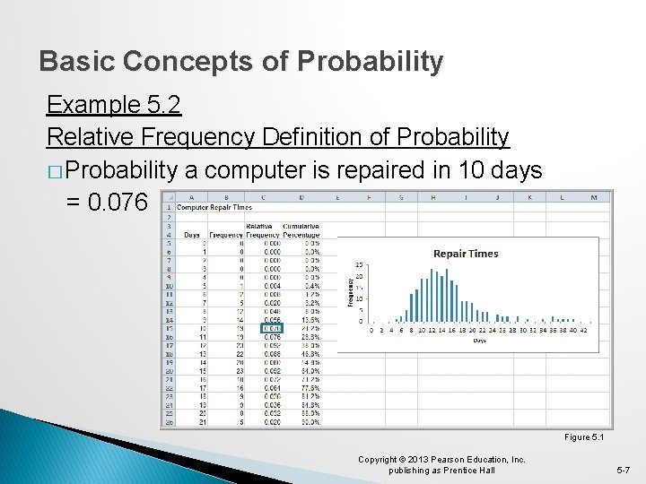
Basic Concepts of Probability Example 5. 2 Relative Frequency Definition of Probability � Probability a computer is repaired in 10 days = 0. 076 Figure 5. 1 Copyright © 2013 Pearson Education, Inc. publishing as Prentice Hall 5 -7

Basic Concepts of Probability Two Basic Facts Govern Probability � The probability associated with any outcome must be between 0 and 1. 0 ≤ P(Oi) ≤ 1 for each outcome Oi � The sum of the probabilities over all possible outcomes must be equal to 1. P(O 1) + P(O 2) + … + P(On) = 1 (n is the number of outcomes in the sample space. ) Copyright © 2013 Pearson Education, Inc. publishing as Prentice Hall 5 -8

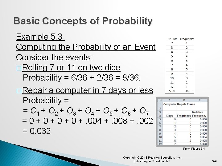
Basic Concepts of Probability Example 5. 3 Computing the Probability of an Event Consider the events: � Rolling 7 or 11 on two dice Probability = 6/36 + 2/36 = 8/36. � Repair a computer in 7 days or less Probability = = O 1 + O 2 + O 3 + O 4 + O 5 + O 6 + O 7 = 0 + 0 +. 004 +. 008 +. 002 = 0. 032 From Figure 5. 1 Copyright © 2013 Pearson Education, Inc. publishing as Prentice Hall 5 -9

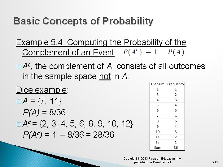
Basic Concepts of Probability Example 5. 4 Computing the Probability of the Complement of an Event � Ac, the complement of A, consists of all outcomes in the sample space not in A. Dice example: � A = {7, 11} P(A) = 8/36 � Ac = {2, 3, 4, 5, 6, 8, 9, 10, 12} P(Ac) = 1 − 8/36 = 28/36 Copyright © 2013 Pearson Education, Inc. publishing as Prentice Hall 5 -10

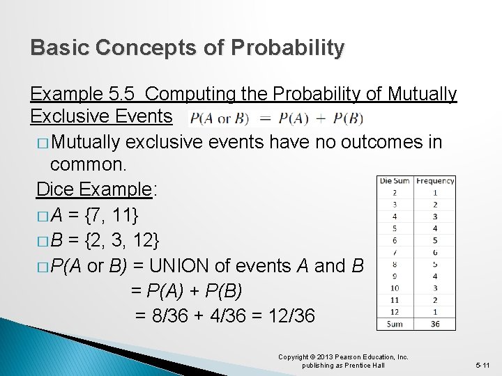
Basic Concepts of Probability Example 5. 5 Computing the Probability of Mutually Exclusive Events � Mutually exclusive events have no outcomes in common. Dice Example: � A = {7, 11} � B = {2, 3, 12} � P(A or B) = UNION of events A and B = P(A) + P(B) = 8/36 + 4/36 = 12/36 Copyright © 2013 Pearson Education, Inc. publishing as Prentice Hall 5 -11

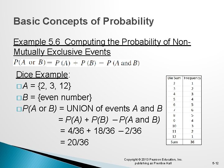
Basic Concepts of Probability Example 5. 6 Computing the Probability of Non. Mutually Exclusive Events Dice Example: � A = {2, 3, 12} � B = {even number} � P(A or B) = UNION of events A and B = P(A) + P(B) − P(A and B) = 4/36 + 18/36 − 2/36 = 20/36 Copyright © 2013 Pearson Education, Inc. publishing as Prentice Hall 5 -12

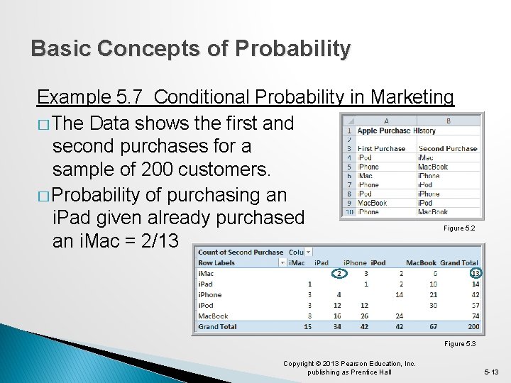
Basic Concepts of Probability Example 5. 7 Conditional Probability in Marketing � The Data shows the first and second purchases for a sample of 200 customers. � Probability of purchasing an i. Pad given already purchased an i. Mac = 2/13 Figure 5. 2 Figure 5. 3 Copyright © 2013 Pearson Education, Inc. publishing as Prentice Hall 5 -13

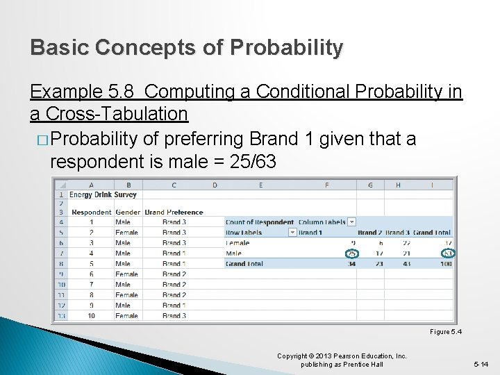
Basic Concepts of Probability Example 5. 8 Computing a Conditional Probability in a Cross-Tabulation � Probability of preferring Brand 1 given that a respondent is male = 25/63 Figure 5. 4 Copyright © 2013 Pearson Education, Inc. publishing as Prentice Hall 5 -14

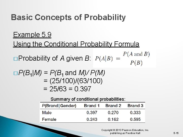
Basic Concepts of Probability Example 5. 9 Using the Conditional Probability Formula � Probability � P(B 1|M) of A given B: = P(B 1 and M)/ P(M) = (25/100)/(63/100) = 25/63 = 0. 397 Summary of conditional probabilities: Copyright © 2013 Pearson Education, Inc. publishing as Prentice Hall 5 -15

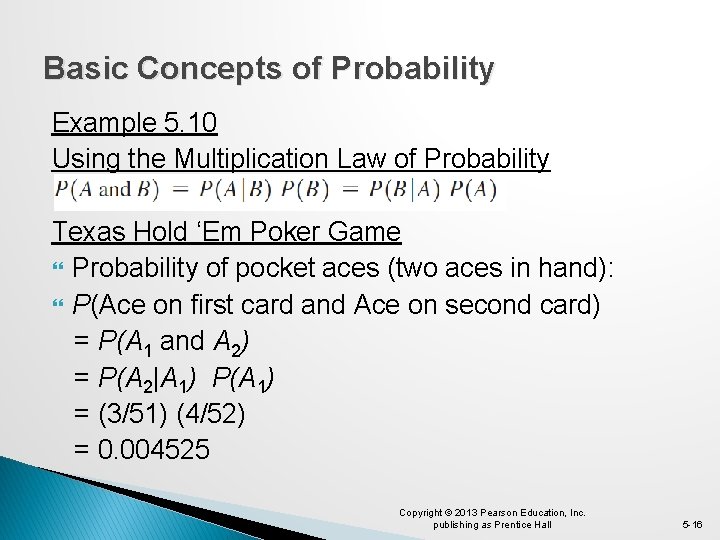
Basic Concepts of Probability Example 5. 10 Using the Multiplication Law of Probability Texas Hold ‘Em Poker Game Probability of pocket aces (two aces in hand): P(Ace on first card and Ace on second card) = P(A 1 and A 2) = P(A 2|A 1) P(A 1) = (3/51) (4/52) = 0. 004525 Copyright © 2013 Pearson Education, Inc. publishing as Prentice Hall 5 -16

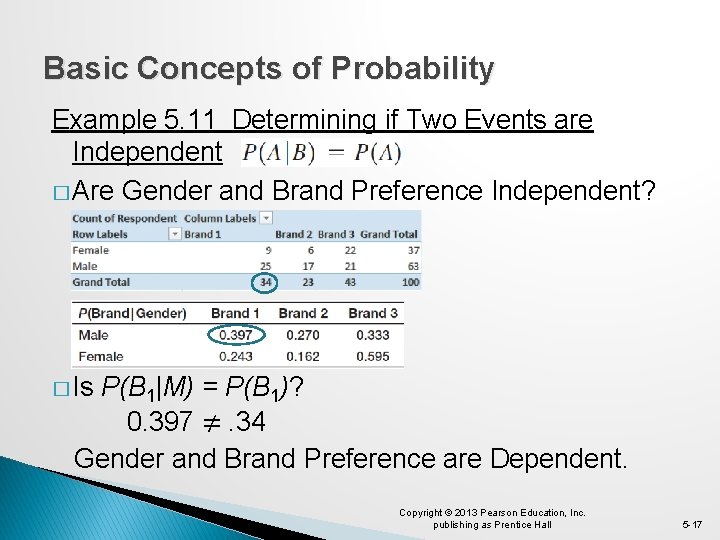
Basic Concepts of Probability Example 5. 11 Determining if Two Events are Independent � Are Gender and Brand Preference Independent? � Is P(B 1|M) = P(B 1)? 0. 397 ≠. 34 Gender and Brand Preference are Dependent. Copyright © 2013 Pearson Education, Inc. publishing as Prentice Hall 5 -17

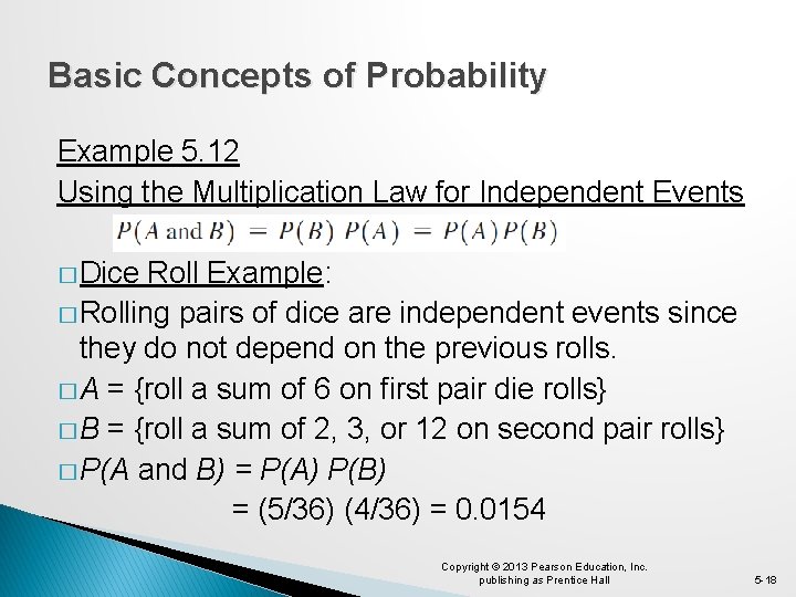
Basic Concepts of Probability Example 5. 12 Using the Multiplication Law for Independent Events � Dice Roll Example: � Rolling pairs of dice are independent events since they do not depend on the previous rolls. � A = {roll a sum of 6 on first pair die rolls} � B = {roll a sum of 2, 3, or 12 on second pair rolls} � P(A and B) = P(A) P(B) = (5/36) (4/36) = 0. 0154 Copyright © 2013 Pearson Education, Inc. publishing as Prentice Hall 5 -18

Random Variables and Probability Distributions A random variable is a numerical description of the outcome of an experiment. A discrete random variable is one for which the number of possible outcomes can be counted. A continuous random variable has outcomes over one or more continuous intervals of real numbers. A probability distribution is a characterization of the possible values that a random variable may assume along with the probability of assuming these values. Copyright © 2013 Pearson Education, Inc. publishing as Prentice Hall 5 -19

Random Variables and Probability Distributions Example 5. 13 Discrete and Continuous Random Variables Examples of Discrete Variables: outcomes of dice rolls whether a customer likes or dislikes a product number of hits on a Web site link today Examples of Continuous Variables: weekly change in DJIA daily temperature time between machine failures Copyright © 2013 Pearson Education, Inc. publishing as Prentice Hall 5 -20

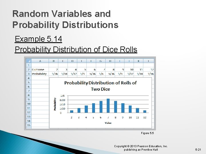
Random Variables and Probability Distributions Example 5. 14 Probability Distribution of Dice Rolls Figure

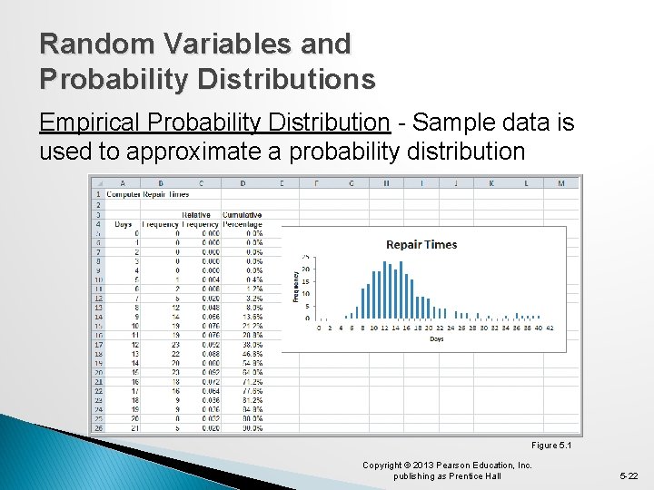
Random Variables and Probability Distributions Empirical Probability Distribution - Sample data is used to approximate a probability distribution Figure 5. 1 Copyright © 2013 Pearson Education, Inc. publishing as Prentice Hall 5 -22

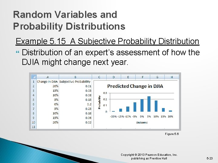
Random Variables and Probability Distributions Example 5. 15 A Subjective Probability Distribution of an expert’s assessment of how the DJIA might change next year. Figure 5. 6 Copyright © 2013 Pearson Education, Inc. publishing as Prentice Hall 5 -23

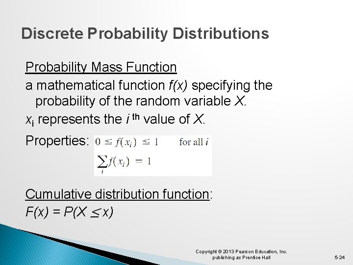
Discrete Probability Distributions Probability Mass Function a mathematical function f(x) specifying the probability of the random variable X. xi represents the i th value of X. Properties: Cumulative distribution function: F(x) = P(X ≤ x) Copyright © 2013 Pearson Education, Inc. publishing as Prentice Hall 5 -24

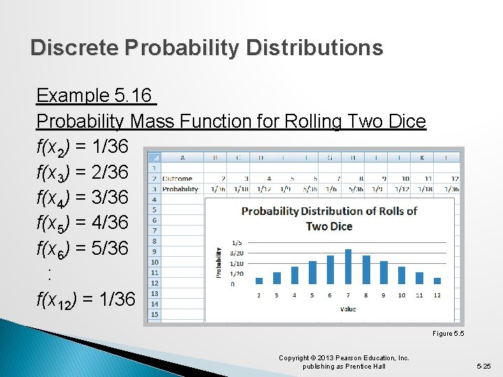
Discrete Probability Distributions Example 5. 16 Probability Mass Function for Rolling Two Dice f(x 2) = 1/36 f(x 3) = 2/36 f(x 4) = 3/36 f(x 5) = 4/36 f(x 6) = 5/36 : f(x 12) = 1/36 Figure 5. 5 Copyright © 2013 Pearson Education, Inc. publishing as Prentice Hall 5 -25

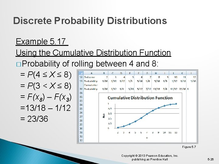
Discrete Probability Distributions Example 5. 17 Using the Cumulative Distribution Function � Probability of rolling between 4 and 8: = P(4 ≤ X ≤ 8) = P(3 < X ≤ 8) = F(x 8) – F(x 3) =13/18 – 1/12 = 23/36 Figure 5. 7 Copyright © 2013 Pearson Education, Inc. publishing as Prentice Hall 5 -26

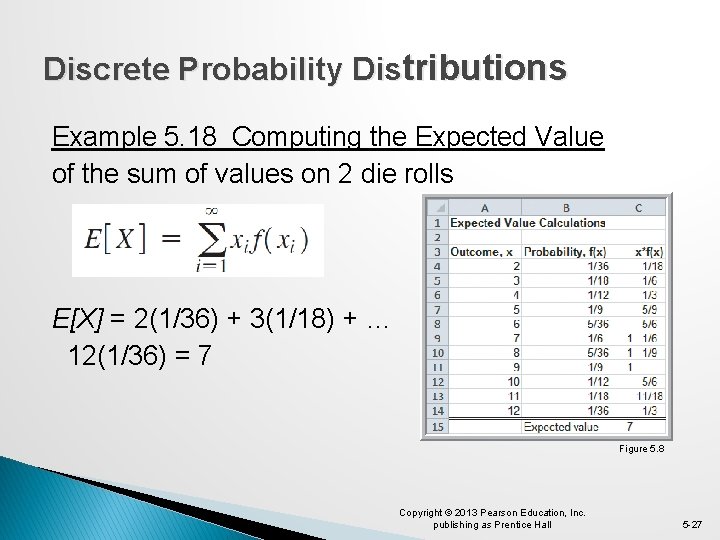
Discrete Probability Distributions Example 5. 18 Computing the Expected Value of the sum of values on 2 die rolls E[X] = 2(1/36) + 3(1/18) + … 12(1/36) = 7 Figure 5. 8 Copyright © 2013 Pearson Education, Inc. publishing as Prentice Hall 5 -27

Discrete Probability Distributions Example 5. 19 Expected Value on Television Apprentice example � Teams were required to select an artist (mainstream or avant-garde) and sell their art for the most money possible. Deal or No Deal example � Contestant had 5 briefcases left with $100, $400, $1000, $50, 000 or $300, 000 in them. � Expected value of briefcases is $70, 300. � Banker offered contestant $80, 000 to quit. Copyright © 2013 Pearson Education, Inc. publishing as Prentice Hall 5 -28

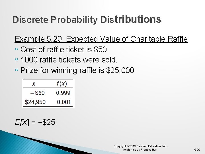
Discrete Probability Distributions Example 5. 20 Expected Value of Charitable Raffle Cost of raffle ticket is $50 1000 raffle tickets were sold. Prize for winning raffle is $25, 000 E[X] = −$25 Copyright © 2013 Pearson Education, Inc. publishing as Prentice Hall 5 -29

Discrete Probability Distributions Example 5. 21 Airline Revenue Management Full and discount airfares are available for a flight. Full-fare ticket costs $560 Discount ticket costs $400 X = ticket price paid p = 0. 75 (the probability of selling a full-fare ticket) E[X] = 0. 75($560) + 0. 25(0) = $420 The airline should not discount full-fare tickets because the expected value of a full-fare ticket is greater than the cost of a discount ticket. Break-even point: $400 = p($560) or p = 0. 714 Copyright © 2013 Pearson Education, Inc. publishing as Prentice Hall 5 -30

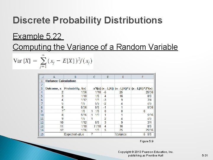
Discrete Probability Distributions Example 5. 22 Computing the Variance of a Random Variable Figure

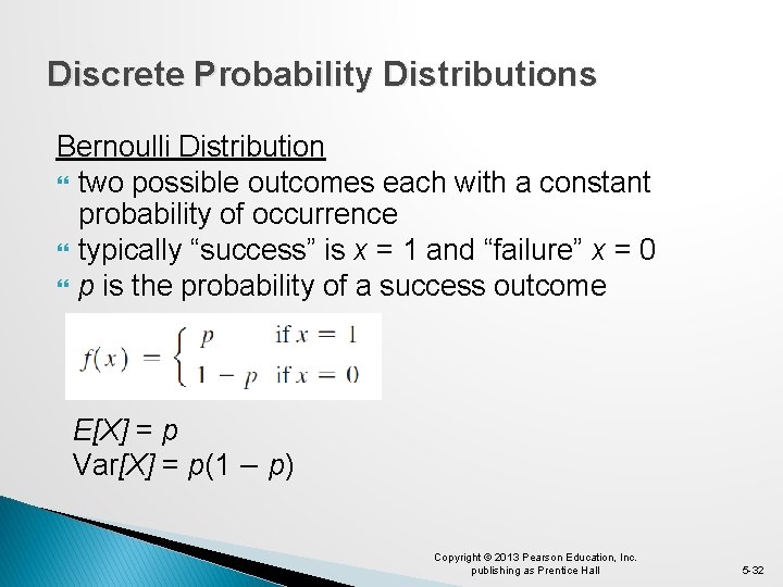
Discrete Probability Distributions Bernoulli Distribution two possible outcomes each with a constant probability of occurrence typically “success” is x = 1 and “failure” x = 0 p is the probability of a success outcome E[X] = p Var[X] = p(1 − p) Copyright © 2013 Pearson Education, Inc. publishing as Prentice Hall 5 -32

Discrete Probability Distributions Example 5. 23 Using the Bernoulli Distribution Model whether an individual responds positively to a telemarketing promotion. � You have a box with 20 red and 80 white marbles. � You ask individuals exposed to the telemarketing promotion to select a marble and then replace it. � If the customer selects a red marble, the customer makes a purchase. � If the customer selects a white marble, the customer does not make a purchase. Copyright © 2013 Pearson Education, Inc. publishing as Prentice Hall 5 -33

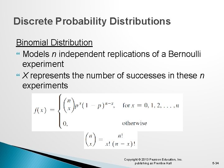
Discrete Probability Distributions Binomial Distribution Models n independent replications of a Bernoulli experiment X represents the number of successes in these n experiments Copyright © 2013 Pearson Education, Inc. publishing as Prentice Hall 5 -34

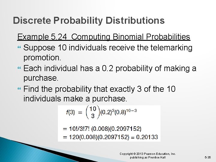
Discrete Probability Distributions Example 5. 24 Computing Binomial Probabilities Suppose 10 individuals receive the telemarking promotion. Each individual has a 0. 2 probability of making a purchase. Find the probability that exactly 3 of the 10 individuals make a purchase. Copyright © 2013 Pearson Education, Inc. publishing as Prentice Hall 5 -35

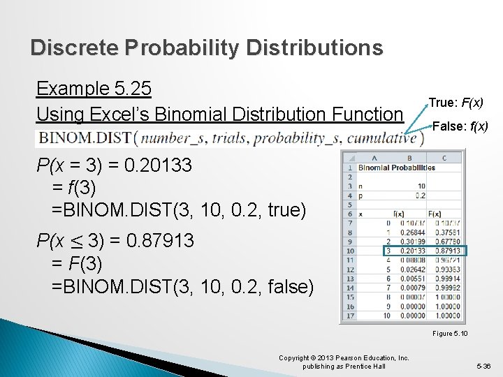
Discrete Probability Distributions Example 5. 25 Using Excel’s Binomial Distribution Function True: F(x) False: f(x) P(x = 3) = 0. 20133 = f(3) =BINOM. DIST(3, 10, 0. 2, true) P(x ≤ 3) = 0. 87913 = F(3) =BINOM. DIST(3, 10, 0. 2, false) Figure 5. 10 Copyright © 2013 Pearson Education, Inc. publishing as Prentice Hall 5 -36

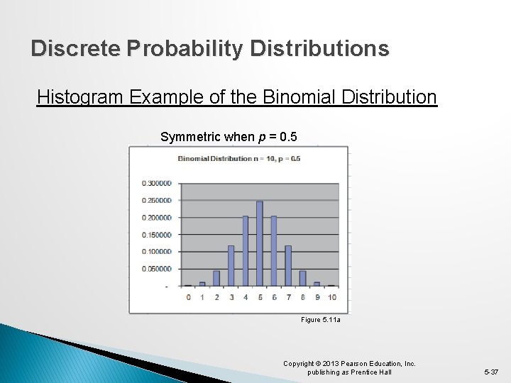
Discrete Probability Distributions Histogram Example of the Binomial Distribution Symmetric when p = 0.

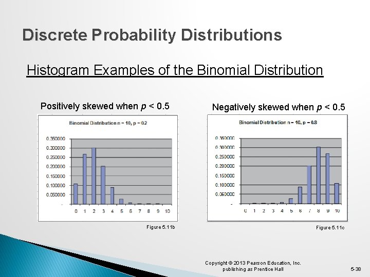
Discrete Probability Distributions Histogram Examples of the Binomial Distribution Positively skewed when p < 0. 5 Negatively skewed when p < 0. 5 Figure 5. 11 b Figure 5. 11 c Copyright © 2013 Pearson Education, Inc. publishing as Prentice Hall 5 -38

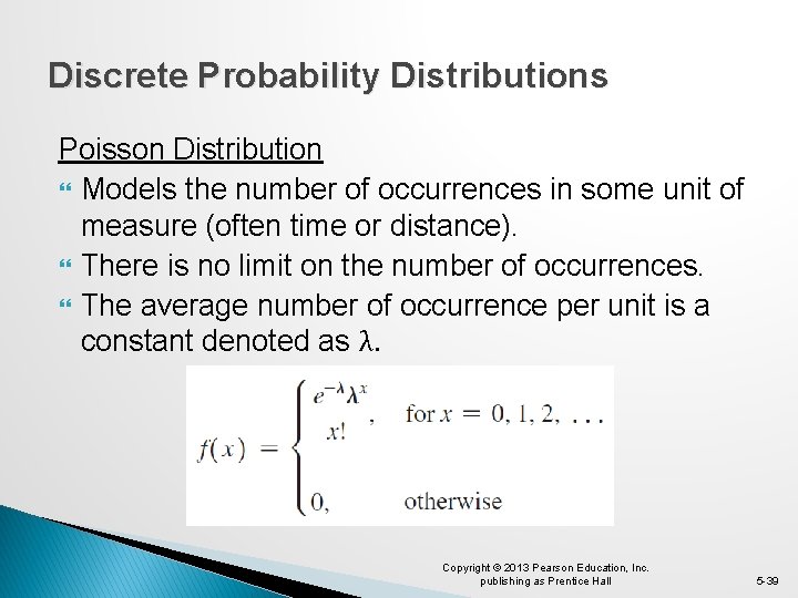
Discrete Probability Distributions Poisson Distribution Models the number of occurrences in some unit of measure (often time or distance). There is no limit on the number of occurrences. The average number of occurrence per unit is a constant denoted as λ. Copyright © 2013 Pearson Education, Inc. publishing as Prentice Hall 5 -39

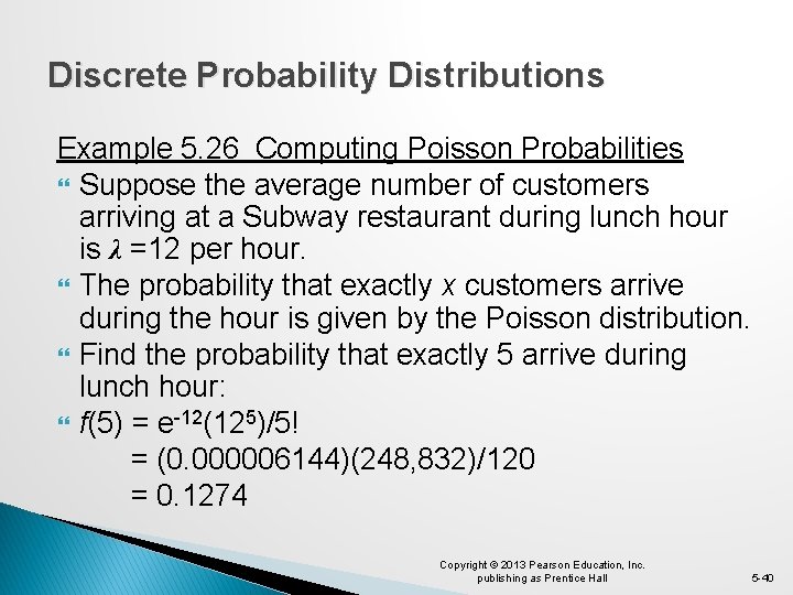
Discrete Probability Distributions Example 5. 26 Computing Poisson Probabilities Suppose the average number of customers arriving at a Subway restaurant during lunch hour is λ =12 per hour. The probability that exactly x customers arrive during the hour is given by the Poisson distribution. Find the probability that exactly 5 arrive during lunch hour: f(5) = e-12(125)/5! = (0. 000006144)(248, 832)/120 = 0. 1274 Copyright © 2013 Pearson Education, Inc. publishing as Prentice Hall 5 -40

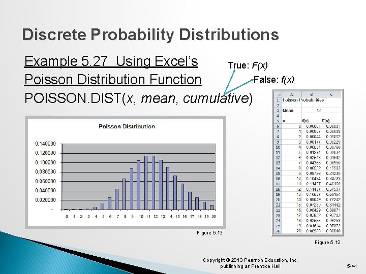
Discrete Probability Distributions Example 5. 27 Using Excel’s True: F(x) False: f(x) Poisson Distribution Function POISSON. DIST(x, mean, cumulative) Figure 5. 13 Figure 5. 12 Copyright © 2013 Pearson Education, Inc. publishing as Prentice Hall 5 -41

Discrete Probability Distributions Analytics in Practice: Using the Poisson Distribution for Modeling Bids on Priceline � Pricing strategies for Kimpton hotels on Priceline is modeled using a Poisson distribution. � The number of bids placed per day 3 days before arrival is f(x) = e-6. 3(6. 3 x)/x!. � Using the model increased sales 11% in one year. Copyright © 2013 Pearson Education, Inc. publishing as Prentice Hall 5 -42

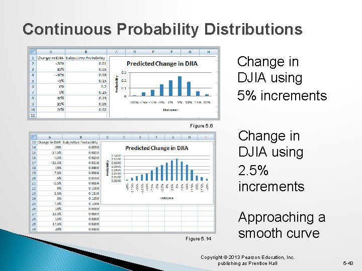
Continuous Probability Distributions Change in DJIA using 5% increments Figure 5. 6 Figure 5. 14 Change in DJIA using 2. 5% increments Approaching a smooth curve Copyright © 2013 Pearson Education, Inc. publishing as Prentice Hall 5 -43

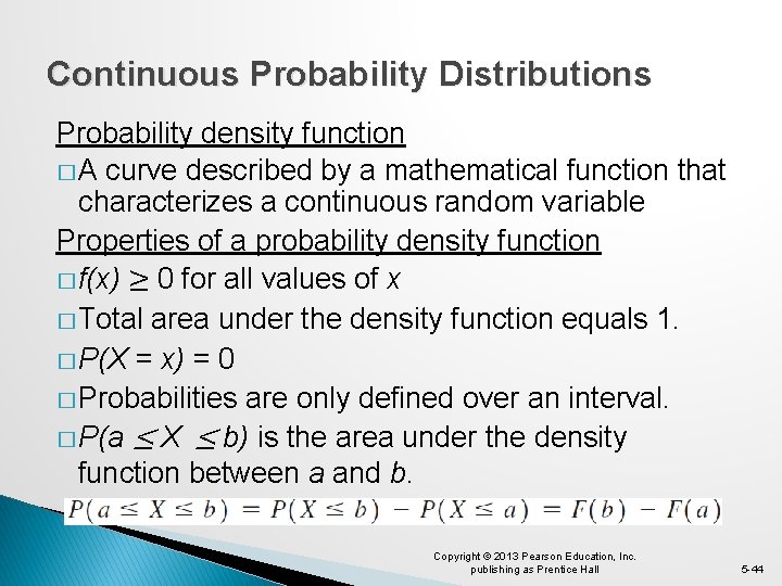
Continuous Probability Distributions Probability density function � A curve described by a mathematical function that characterizes a continuous random variable Properties of a probability density function � f(x) ≥ 0 for all values of x � Total area under the density function equals 1. � P(X = x) = 0 � Probabilities are only defined over an interval. � P(a ≤ X ≤ b) is the area under the density function between a and b. Copyright © 2013 Pearson Education, Inc. publishing as Prentice Hall 5 -44

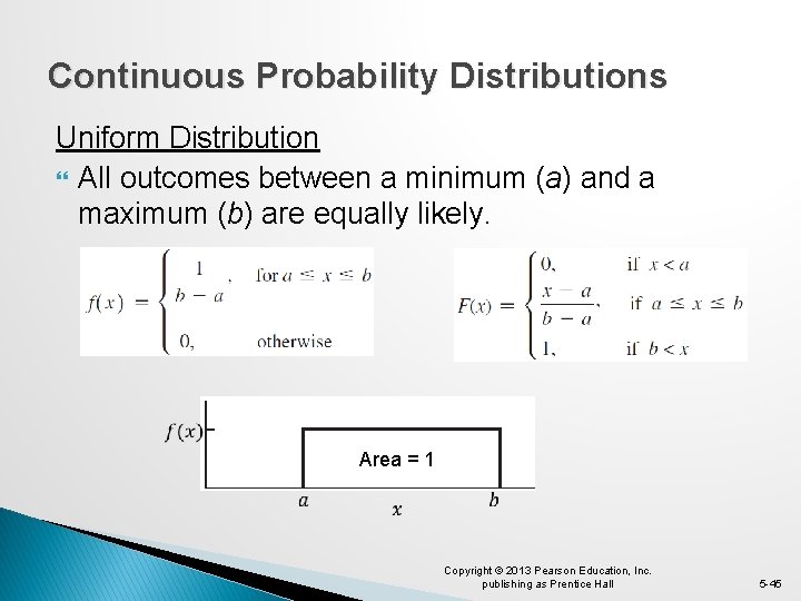
Continuous Probability Distributions Uniform Distribution All outcomes between a minimum (a) and a maximum (b) are equally likely. Area = 1 Copyright © 2013 Pearson Education, Inc. publishing as Prentice Hall 5 -45

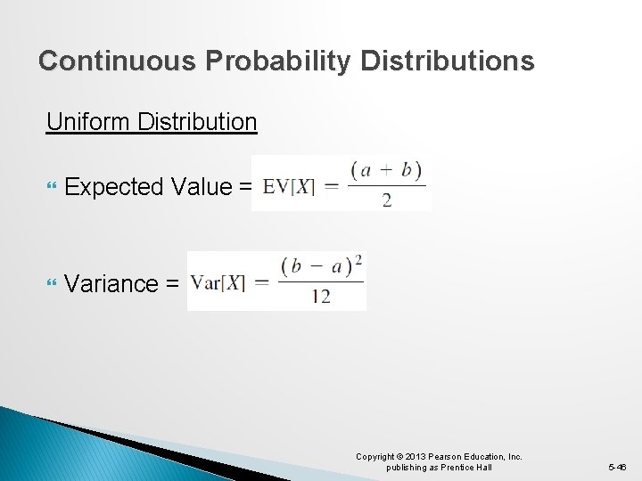
Continuous Probability Distributions Uniform Distribution Expected Value = Variance = Copyright © 2013 Pearson

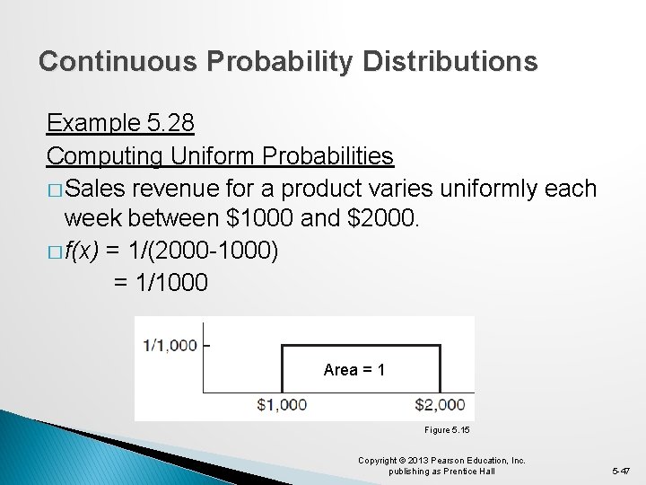
Continuous Probability Distributions Example 5. 28 Computing Uniform Probabilities � Sales revenue for a product varies uniformly each week between $1000 and $2000. � f(x) = 1/(2000 -1000) = 1/1000 Area = 1 Figure 5. 15 Copyright © 2013 Pearson Education, Inc. publishing as Prentice Hall 5 -47

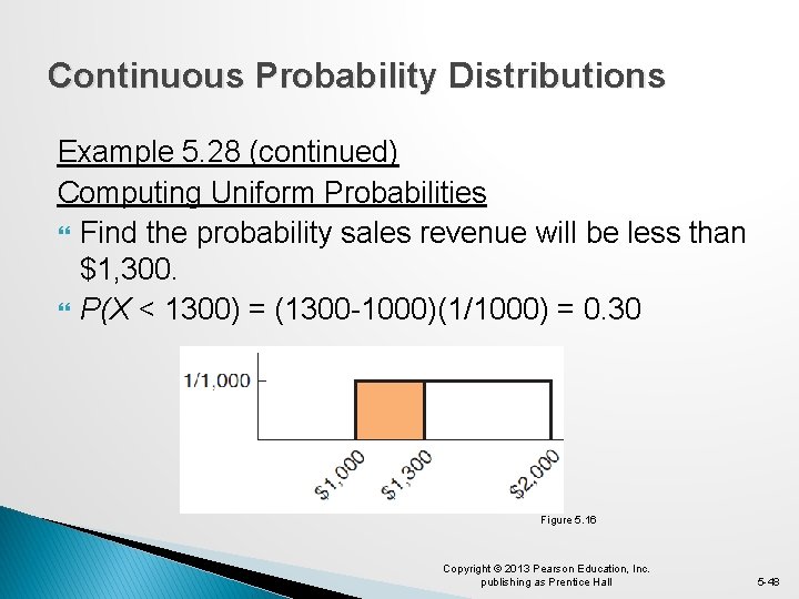
Continuous Probability Distributions Example 5. 28 (continued) Computing Uniform Probabilities Find the probability sales revenue will be less than $1, 300. P(X < 1300) = (1300 -1000)(1/1000) = 0. 30 Figure 5. 16 Copyright © 2013 Pearson Education, Inc. publishing as Prentice Hall 5 -48

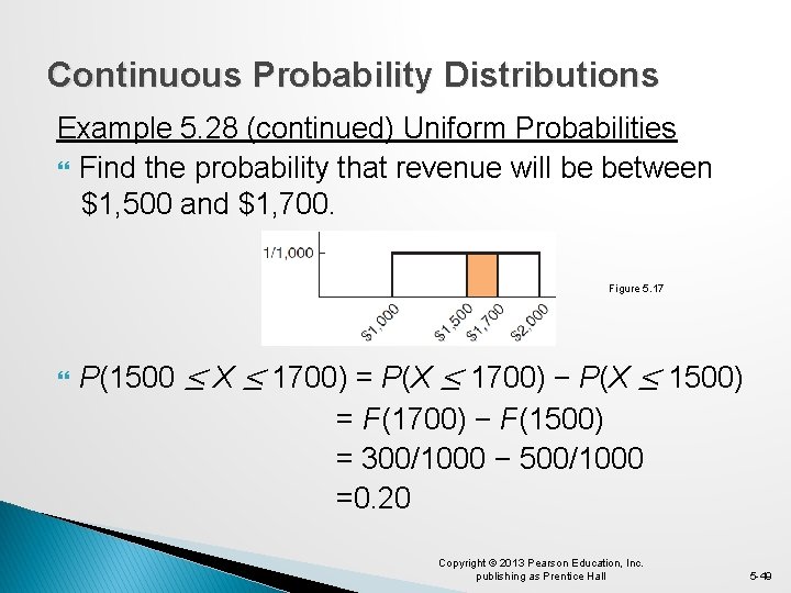
Continuous Probability Distributions Example 5. 28 (continued) Uniform Probabilities Find the probability that revenue will be between $1, 500 and $1, 700. Figure 5. 17 P(1500 ≤ X ≤ 1700) = P(X ≤ 1700) − P(X ≤ 1500) = F(1700) − F(1500) = 300/1000 − 500/1000 =0. 20 Copyright © 2013 Pearson Education, Inc. publishing as Prentice Hall 5 -49

Continuous Probability Distributions Normal Distribution - f(x) is a bell-shaped curve - Characterized by 2 parameters (mean) (standard deviation) - Properties 1. Symmetric 2. Mean = Median = Mode 3. Unbounded 4. Empirical rules apply Copyright © 2013 Pearson Education, Inc. publishing as Prentice Hall 5 -50

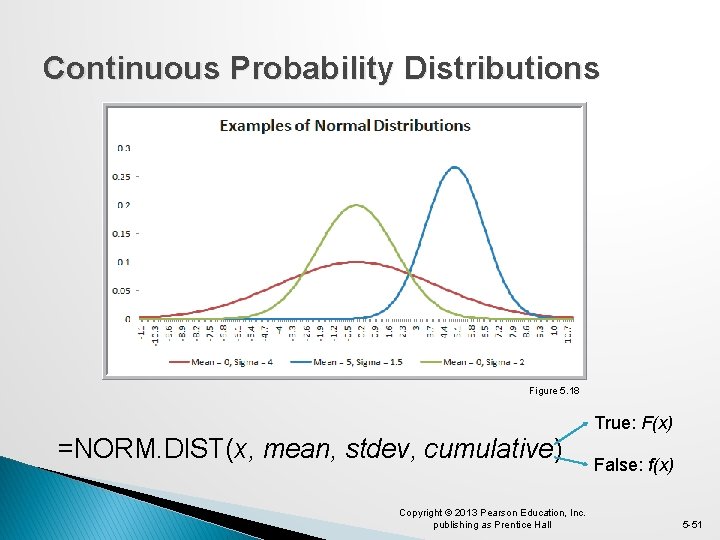
Continuous Probability Distributions Figure 5. 18 True: F(x) =NORM. DIST(x, mean, stdev, cumulative) Copyright

Continuous Probability Distributions Example 5. 29 Using NORM. DIST to Compute Normal Probabilities � The distribution for customer demand (units per month) is normal with: mean = 750 stdev. = 100 � Find the probability that demand will be: a) at most 900 units/month b) exceed 700 units/month c) be between 700 and 900 units/month Copyright © 2013 Pearson Education, Inc. publishing as Prentice Hall 5 -52

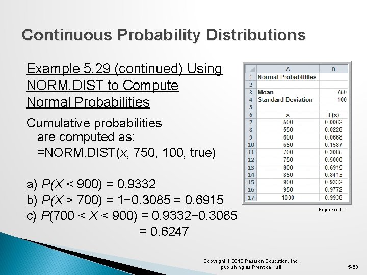
Continuous Probability Distributions Example 5. 29 (continued) Using NORM. DIST to Compute Normal Probabilities Cumulative probabilities are computed as: =NORM. DIST(x, 750, 100, true) a) P(X < 900) = 0. 9332 b) P(X > 700) = 1− 0. 3085 = 0. 6915 c) P(700 < X < 900) = 0. 9332− 0. 3085 = 0. 6247 Copyright © 2013 Pearson Education, Inc. publishing as Prentice Hall Figure 5. 19 5 -53

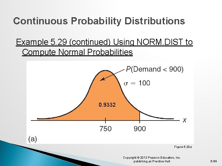
Continuous Probability Distributions Example 5. 29 (continued) Using NORM. DIST to Compute Normal Probabilities 0. 9332 Figure 5. 20 a Copyright © 2013 Pearson Education, Inc. publishing as Prentice Hall 5 -54

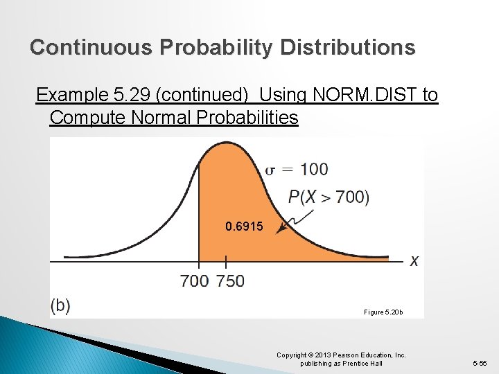
Continuous Probability Distributions Example 5. 29 (continued) Using NORM. DIST to Compute Normal Probabilities 0. 6915 Figure 5. 20 b Copyright © 2013 Pearson Education, Inc. publishing as Prentice Hall 5 -55

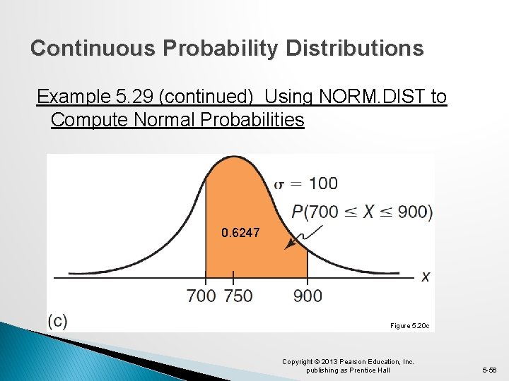
Continuous Probability Distributions Example 5. 29 (continued) Using NORM. DIST to Compute Normal Probabilities 0. 6247 Figure 5. 20 c Copyright © 2013 Pearson Education, Inc. publishing as Prentice Hall 5 -56

Continuous Probability Distributions Example 5. 30 Using the NORM. INV Function =NORM. INV(probability, mean, stdev) provides the x value with F(x)= probability What level of demand would be exceeded at most 10% of the time? Find x such that F(x) = 90% = NORM. INV(0. 90, 750, 100) results in x = 878. 155 Copyright © 2013 Pearson Education, Inc. publishing as Prentice Hall 5 -57

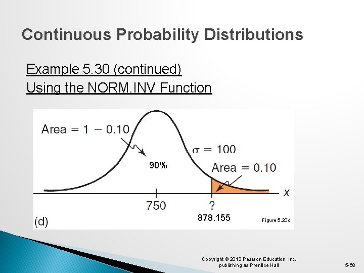
Continuous Probability Distributions Example 5. 30 (continued) Using the NORM. INV Function 90% 878.

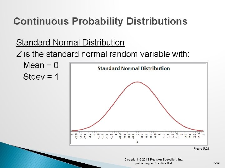
Continuous Probability Distributions Standard Normal Distribution Z is the standard normal random variable with: Mean = 0 Stdev = 1 Figure 5. 21 Copyright © 2013 Pearson Education, Inc. publishing as Prentice Hall 5 -59

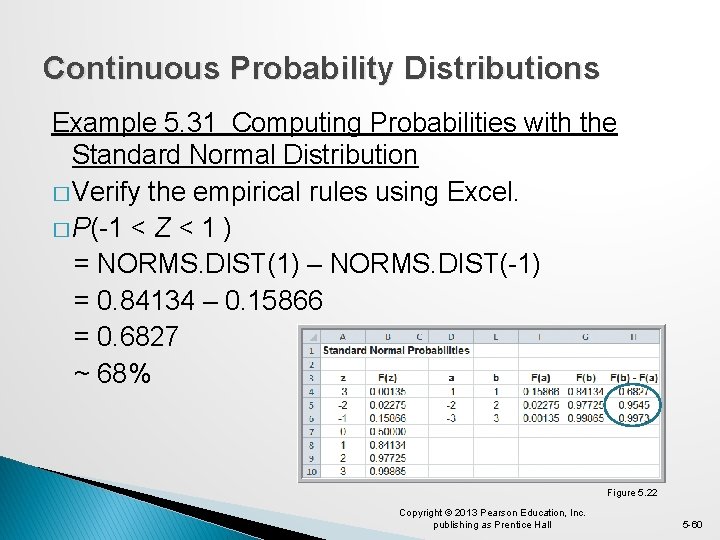
Continuous Probability Distributions Example 5. 31 Computing Probabilities with the Standard Normal Distribution � Verify the empirical rules using Excel. � P(-1 < Z < 1 ) = NORMS. DIST(1) – NORMS. DIST(-1) = 0. 84134 – 0. 15866 = 0. 6827 ~ 68% Figure 5. 22 Copyright © 2013 Pearson Education, Inc. publishing as Prentice Hall 5 -60

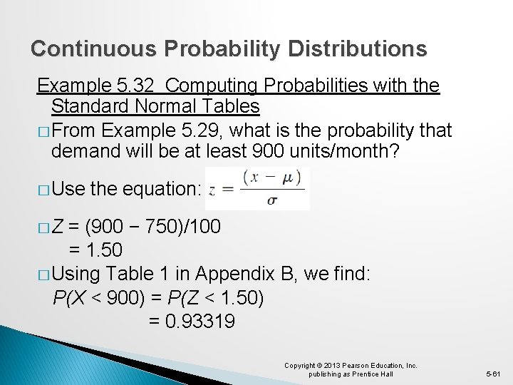
Continuous Probability Distributions Example 5. 32 Computing Probabilities with the Standard Normal Tables � From Example 5. 29, what is the probability that demand will be at least 900 units/month? � Use the equation: �Z = (900 − 750)/100 = 1. 50 � Using Table 1 in Appendix B, we find: P(X < 900) = P(Z < 1. 50) = 0. 93319 Copyright © 2013 Pearson Education, Inc. publishing as Prentice Hall 5 -61

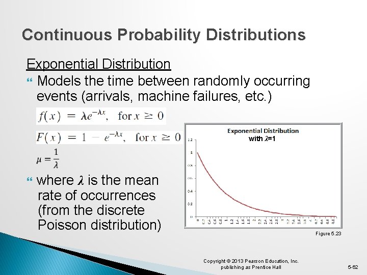
Continuous Probability Distributions Exponential Distribution Models the time between randomly occurring events (arrivals, machine failures, etc. ) with λ=1 where λ is the mean rate of occurrences (from the discrete Poisson distribution) Figure 5. 23 Copyright © 2013 Pearson Education, Inc. publishing as Prentice Hall 5 -62

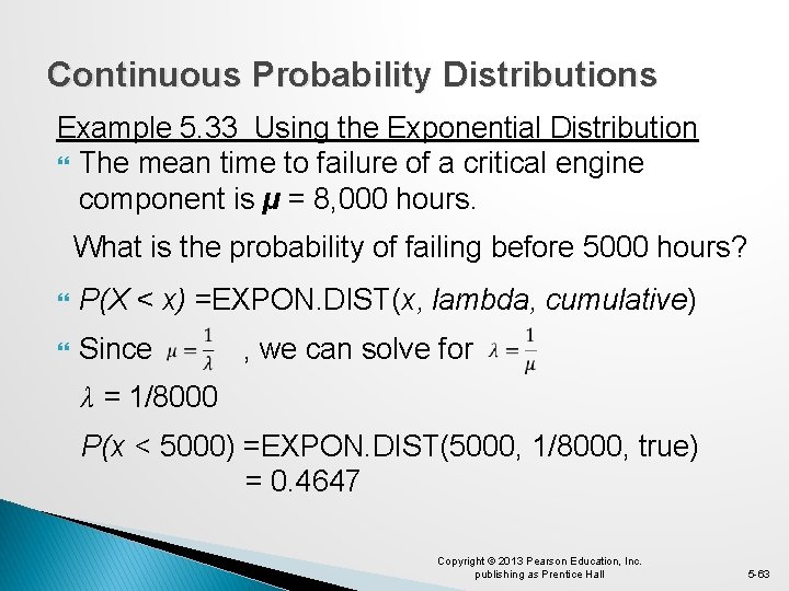
Continuous Probability Distributions Example 5. 33 Using the Exponential Distribution The mean time to failure of a critical engine component is µ = 8, 000 hours. What is the probability of failing before 5000 hours? P(X < x) =EXPON. DIST(x, lambda, cumulative) Since , we can solve for λ = 1/8000 P(x < 5000) =EXPON. DIST(5000, 1/8000, true) = 0. 4647 Copyright © 2013 Pearson Education, Inc. publishing as Prentice Hall 5 -63

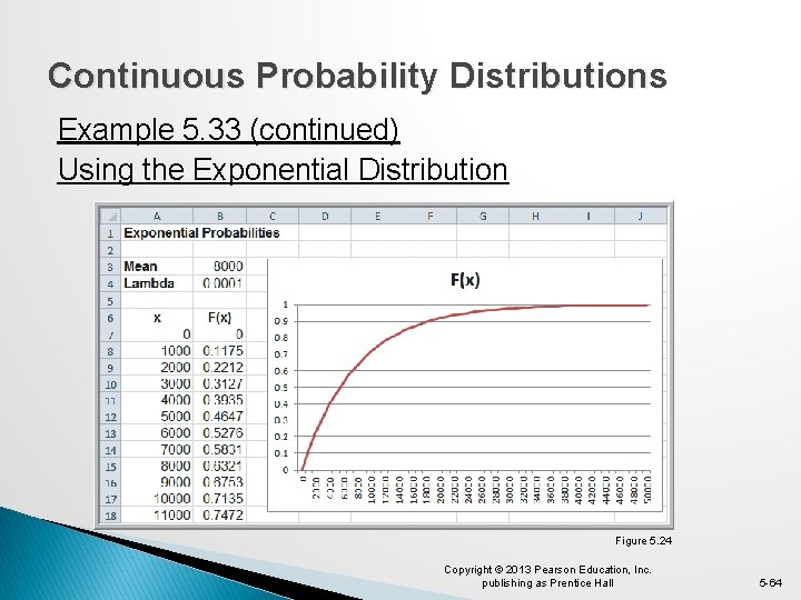
Continuous Probability Distributions Example 5. 33 (continued) Using the Exponential Distribution Figure 5. 24

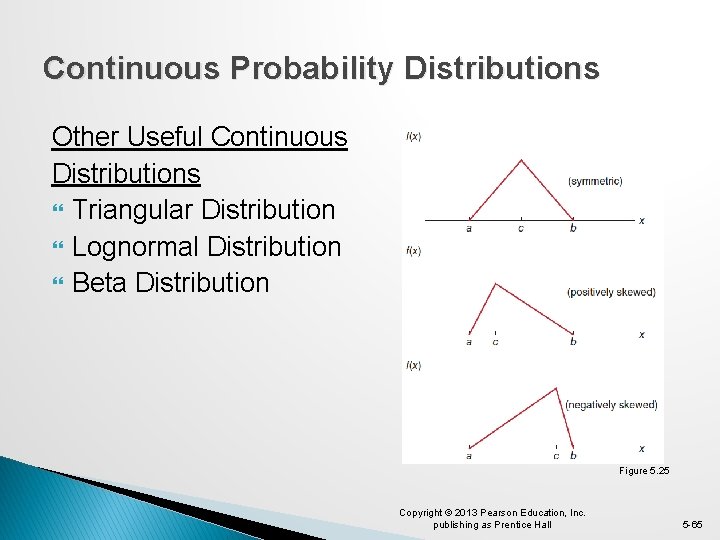
Continuous Probability Distributions Other Useful Continuous Distributions Triangular Distribution Lognormal Distribution Beta Distribution Figure 5. 25 Copyright © 2013 Pearson Education, Inc. publishing as Prentice Hall 5 -65

Random Sampling from Probability Distributions � Many application in Business Analytics require random samples from specific probability distributions. � For example, cumulative discounted cash flow can be described using probability distributions for sales, sales growth rate, operating expenses, and inflation factors (all uncertain variables). � Random numbers are the basis for generating random samples from probability distributions. � Random numbers are uniformly distributed on the interval from 0 to 1. Copyright © 2013 Pearson Education, Inc. publishing as Prentice Hall 5 -66

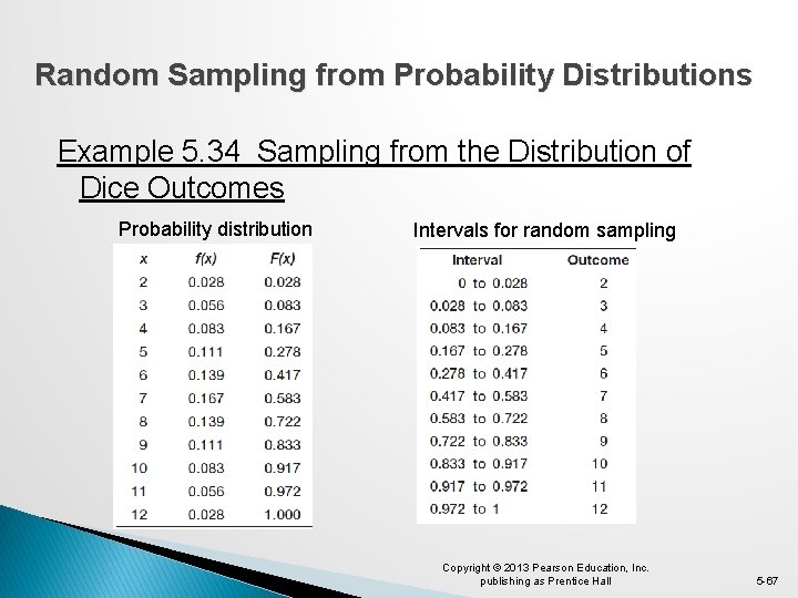
Random Sampling from Probability Distributions Example 5. 34 Sampling from the Distribution of Dice Outcomes Probability distribution Intervals for random sampling Copyright © 2013 Pearson Education, Inc. publishing as Prentice Hall 5 -67

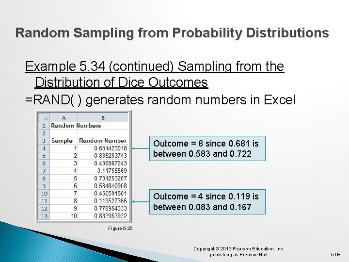
Random Sampling from Probability Distributions Example 5. 34 (continued) Sampling from the Distribution of Dice Outcomes =RAND( ) generates random numbers in Excel Outcome = 8 since 0. 681 is between 0. 583 and 0. 722 Outcome = 4 since 0. 119 is between 0. 083 and 0. 167 Figure 5. 26 Copyright © 2013 Pearson Education, Inc. publishing as Prentice Hall 5 -68

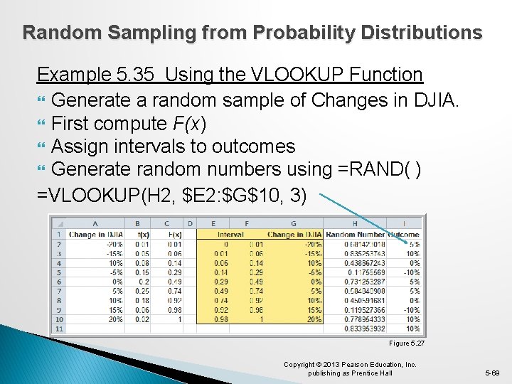
Random Sampling from Probability Distributions Example 5. 35 Using the VLOOKUP Function Generate a random sample of Changes in DJIA. First compute F(x) Assign intervals to outcomes Generate random numbers using =RAND( ) =VLOOKUP(H 2, $E 2: $G$10, 3) Figure 5. 27 Copyright © 2013 Pearson Education, Inc. publishing as Prentice Hall 5 -69

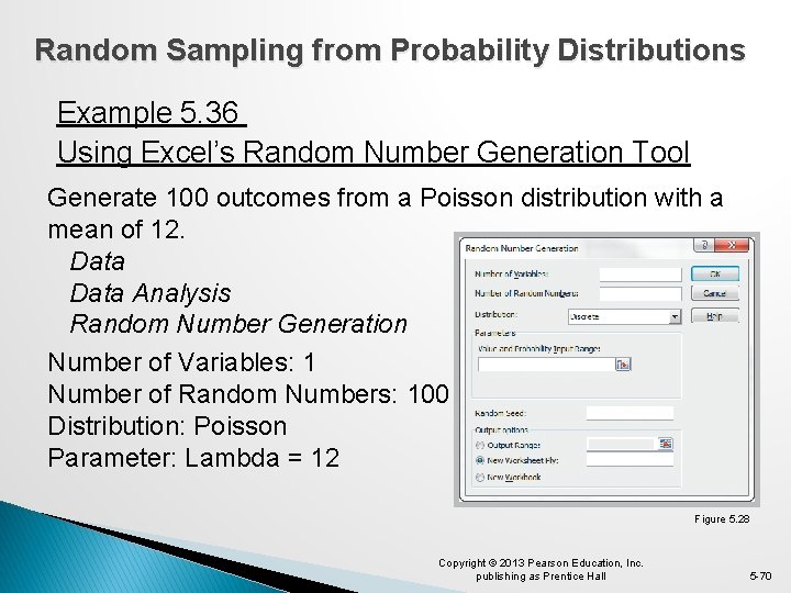
Random Sampling from Probability Distributions Example 5. 36 Using Excel’s Random Number Generation Tool Generate 100 outcomes from a Poisson distribution with a mean of 12. Data Analysis Random Number Generation Number of Variables: 1 Number of Random Numbers: 100 Distribution: Poisson Parameter: Lambda = 12 Figure 5. 28 Copyright © 2013 Pearson Education, Inc. publishing as Prentice Hall 5 -70

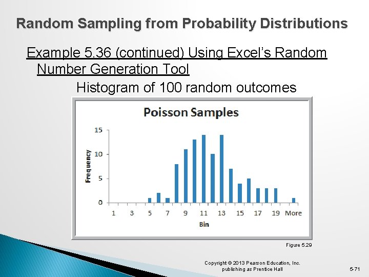
Random Sampling from Probability Distributions Example 5. 36 (continued) Using Excel’s Random Number Generation Tool Histogram of 100 random outcomes Figure 5. 29 Copyright © 2013 Pearson Education, Inc. publishing as Prentice Hall 5 -71

Random Sampling from Probability Distributions available in Excel’s Data Analysis Toolpak under Random Number Generation � Bernoulli � Binomial � Discrete � Normal � Patterned � Poisson � Uniform Copyright © 2013 Pearson Education, Inc. publishing as Prentice Hall 5 -72

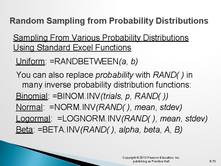
Random Sampling from Probability Distributions Sampling From Various Probability Distributions Using Standard Excel Functions Uniform: =RANDBETWEEN(a, b) You can also replace probability with RAND( ) in many inverse probability distribution functions: Binomial: =BINOM. INV(trials, p, RAND( )) Normal: =NORM. INV(RAND( ), mean, stdev) Logormal: =LOGNORM. INV(RAND( ), mean, stdev) Beta: =BETA. INV(RAND( ), alpha, beta, A, B) Copyright © 2013 Pearson Education, Inc. publishing as Prentice Hall 5 -73

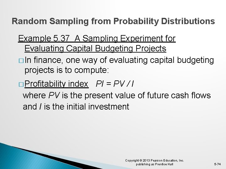
Random Sampling from Probability Distributions Example 5. 37 A Sampling Experiment for Evaluating Capital Budgeting Projects � In finance, one way of evaluating capital budgeting projects is to compute: � Profitability index PI = PV / I where PV is the present value of future cash flows and I is the initial investment Copyright © 2013 Pearson Education, Inc. publishing as Prentice Hall 5 -74

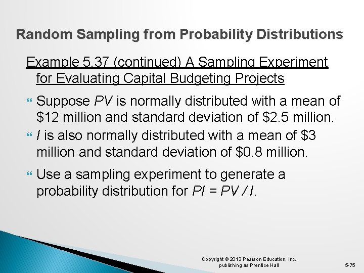
Random Sampling from Probability Distributions Example 5. 37 (continued) A Sampling Experiment for Evaluating Capital Budgeting Projects Suppose PV is normally distributed with a mean of $12 million and standard deviation of $2. 5 million. I is also normally distributed with a mean of $3 million and standard deviation of $0. 8 million. Use a sampling experiment to generate a probability distribution for PI = PV / I. Copyright © 2013 Pearson Education, Inc. publishing as Prentice Hall 5 -75

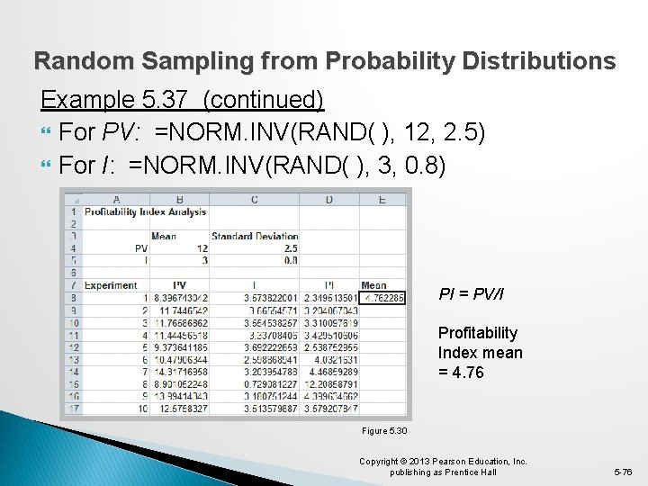
Random Sampling from Probability Distributions Example 5. 37 (continued) For PV: =NORM. INV(RAND( ), 12, 2. 5) For I: =NORM. INV(RAND( ), 3, 0. 8) PI = PV/I Profitability Index mean = 4. 76 Figure 5. 30 Copyright © 2013 Pearson Education, Inc. publishing as Prentice Hall 5 -76

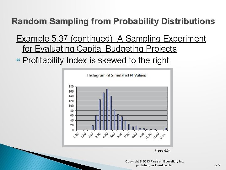
Random Sampling from Probability Distributions Example 5. 37 (continued) A Sampling Experiment for Evaluating Capital Budgeting Projects Profitability Index is skewed to the right Figure 5. 31 Copyright © 2013 Pearson Education, Inc. publishing as Prentice Hall 5 -77

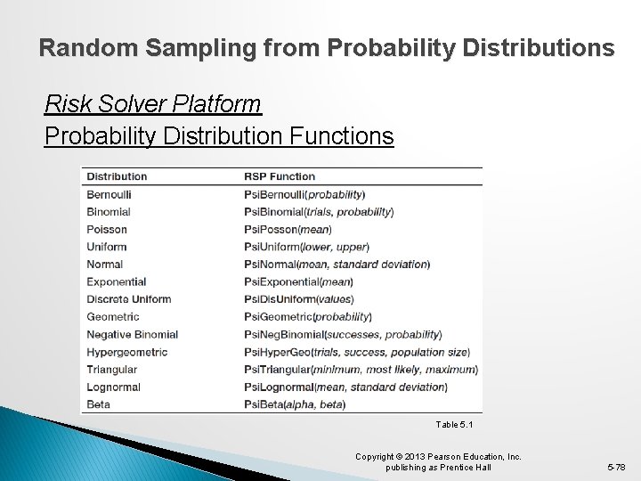
Random Sampling from Probability Distributions Risk Solver Platform Probability Distribution Functions Table 5. 1

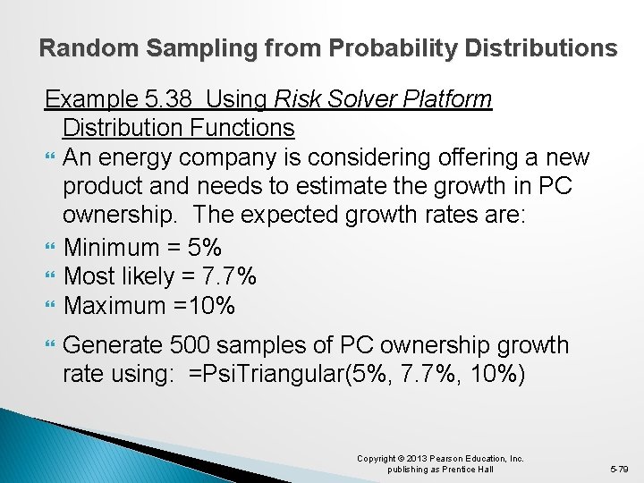
Random Sampling from Probability Distributions Example 5. 38 Using Risk Solver Platform Distribution Functions An energy company is considering offering a new product and needs to estimate the growth in PC ownership. The expected growth rates are: Minimum = 5% Most likely = 7. 7% Maximum =10% Generate 500 samples of PC ownership growth rate using: =Psi. Triangular(5%, 7. 7%, 10%) Copyright © 2013 Pearson Education, Inc. publishing as Prentice Hall 5 -79

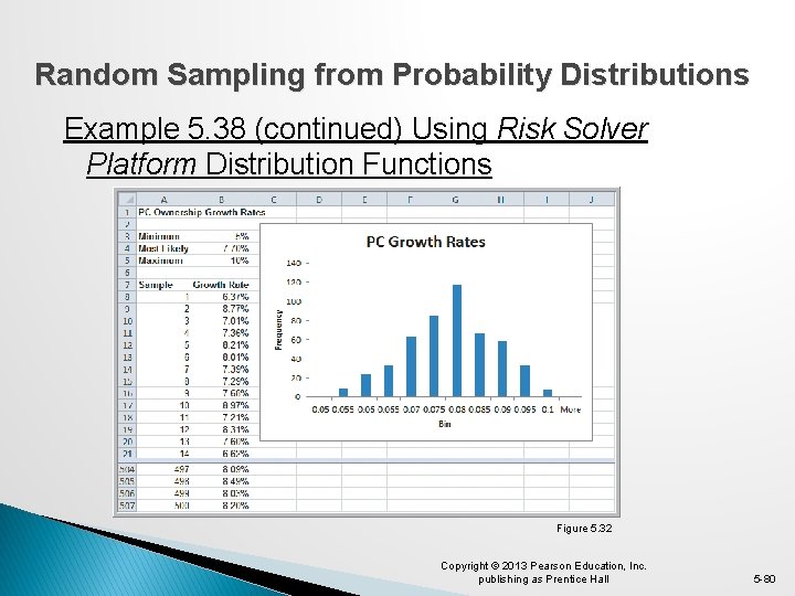
Random Sampling from Probability Distributions Example 5. 38 (continued) Using Risk Solver Platform Distribution Functions Figure 5. 32 Copyright © 2013 Pearson Education, Inc. publishing as Prentice Hall 5 -80

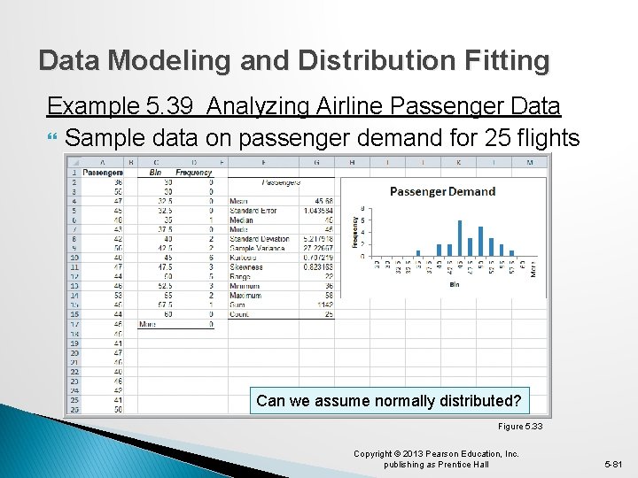
Data Modeling and Distribution Fitting Example 5. 39 Analyzing Airline Passenger Data Sample data on passenger demand for 25 flights Can we assume normally distributed? Figure 5. 33 Copyright © 2013 Pearson Education, Inc. publishing as Prentice Hall 5 -81

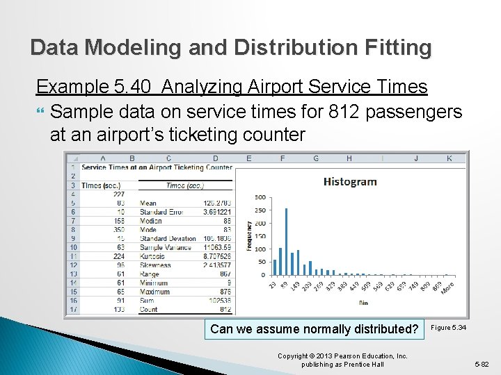
Data Modeling and Distribution Fitting Example 5. 40 Analyzing Airport Service Times Sample data on service times for 812 passengers at an airport’s ticketing counter Can we assume normally distributed? Copyright © 2013 Pearson Education, Inc. publishing as Prentice Hall Figure 5. 34 5 -82

Data Modeling and Distribution Fitting Goodness of Fit The basis for fitting data to a probability distribution Attempts to draw conclusions about the nature of the distribution Three statistics measure goodness of fit: Chi-square Kolmogorov-Smirnov Anderson-Darling Copyright © 2013 Pearson Education, Inc. publishing as Prentice Hall 5 -83

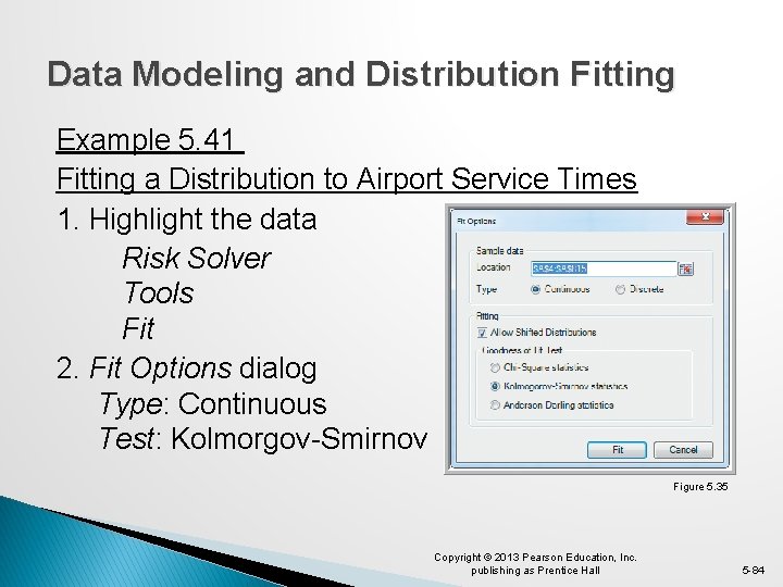
Data Modeling and Distribution Fitting Example 5. 41 Fitting a Distribution to Airport Service Times 1. Highlight the data Risk Solver Tools Fit 2. Fit Options dialog Type: Continuous Test: Kolmorgov-Smirnov Figure 5. 35 Copyright © 2013 Pearson Education, Inc. publishing as Prentice Hall 5 -84

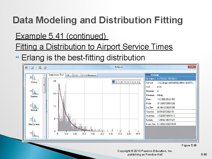
Data Modeling and Distribution Fitting Example 5. 41 (continued) Fitting a Distribution to Airport Service Times Erlang is the best-fitting distribution Figure 5. 36 Copyright © 2013 Pearson Education, Inc. publishing as Prentice Hall 5 -85

Data Modeling and Distribution Fitting Analytics in Practice: The Value of Good Data Modeling in Advertising Gross’s model: A mathematical model that relates the relative contributions of creative and media dollars to total advertising effectiveness. Often used to identify the best number of ads to purchase. Analysis found that the optimal number of ads can vary significantly depending on the shape of the distribution of effectiveness for a single ad. Copyright © 2013 Pearson Education, Inc. publishing as Prentice Hall 5 -86

Chapter 5 – Key Terms Bernoulli distribution Binomial distribution Complement Conditional probability Continuous random variable Cumulative distribution function Discrete random variable Discrete uniform distribution Empirical probability distribution Event Expected value Experiment Exponential distribution Goodness of fit Independent events Copyright © 2013 Pearson Education, Inc. publishing as Prentice Hall 5 -87

Chapter 5 – Key Terms (continued) Multiplication law of probability Mutually exclusive Normal distribution Outcome Poisson distribution Probability density function Probability distribution Probability mass function Random number seed Random variable Random variate Sample space Standard normal distribution Uniform distribution Union Copyright © 2013 Pearson Education, Inc. publishing as Prentice Hall 5 -88

Case Study Performance Lawn Equipment (5) Recall that PLE produces lawnmowers and a medium size diesel power lawn tractor. Determine probability distributions appropriate for modeling mower failures and blade weights. Determine the sampling distribution of the mean mower failures for a sample size of 100. Determine the sampling distribution of the proportion blade weights below specification for a sample size of 350. Analyze your results and write up a formal report. Copyright © 2013 Pearson Education, Inc. publishing as Prentice Hall 5 -89