Chapter 5 Part B Spatial Autocorrelation and regression

Chapter 5 Part B: Spatial Autocorrelation and regression modelling www. spatialanalysisonline. com

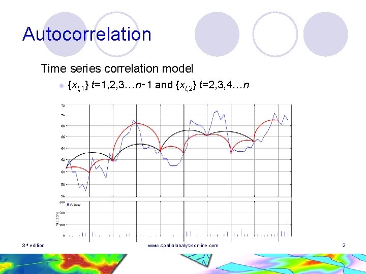
Autocorrelation Time series correlation model l 3 rd edition {xt, 1} t=1, 2, 3…n‑ 1 and {xt, 2} t=2, 3, 4…n www. spatialanalysisonline. com 2

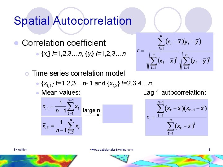
Spatial Autocorrelation l Correlation coefficient l ¡ {xi} i=1, 2, 3…n, {yi} i=1, 2, 3…n Time series correlation model l l {xt, 1} t=1, 2, 3…n‑ 1 and {xt, 2} t=2, 3, 4…n Mean values: Lag 1 autocorrelation: large n 3 rd edition www. spatialanalysisonline. com 3

Spatial Autocorrelation l Classical statistical model assumptions l Independence vs dependence in time and space l Tobler’s first law: “All things are related, but nearby things are more related than distant things” l Spatial dependence and autocorrelation l Correlation and Correlograms 3 rd edition www. spatialanalysisonline. com 4

Spatial Autocorrelation l Covariance and autocovariance l Lags – fixed or variable interval l Correlograms and range l Stationary and non-stationary patterns l Outliers l Extending concept to spatial domain ¡ Transects ¡ Neighbourhoods 3 rd edition and distance-based models www. spatialanalysisonline. com 5

Spatial Autocorrelation l Global spatial autocorrelation ¡ Dataset issues: regular grids; irregular lattice (zonal) datasets; point samples Simple binary coded regular grids – use of Joins counts l Irregular grids and lattices – extension to x, y, z data representation l Use of x, y, z model for point datasets l l Local spatial autocorrelation ¡ Disaggregating 3 rd edition global models www. spatialanalysisonline. com 6

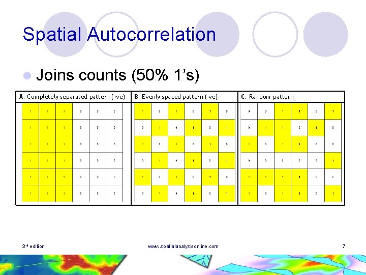
Spatial Autocorrelation l Joins counts (50% 1’s) A. Completely separated pattern (+ve) 3 rd edition B. Evenly spaced pattern (-ve) www. spatialanalysisonline. com C. Random pattern 7

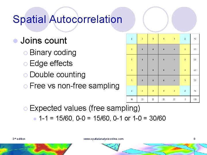
Spatial Autocorrelation l Joins count ¡ Binary coding ¡ Edge effects ¡ Double counting ¡ Free vs non-free sampling ¡ Expected l 3 rd edition values (free sampling) 1 -1 = 15/60, 0 -0 = 15/60, 0 -1 or 1 -0 = 30/60 www. spatialanalysisonline. com 8

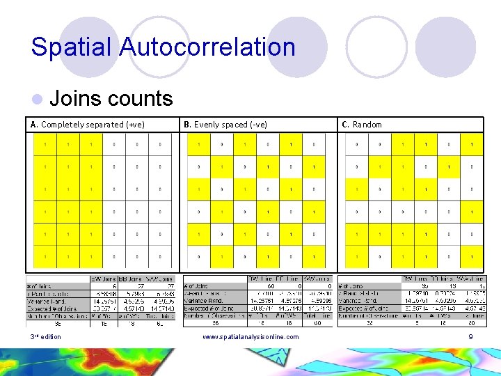
Spatial Autocorrelation l Joins counts A. Completely separated (+ve) 3 rd edition B. Evenly spaced (-ve) www. spatialanalysisonline. com C. Random 9

Spatial Autocorrelation l Joins count – some issues ¡ Multiple z-scores ¡ Binary or k-class data ¡ Rook’s move vs other moves ¡ First order lag vs higher orders ¡ Equal vs unequal weights ¡ Regular grids vs other datasets ¡ Global vs local statistics ¡ Sensitivity to model components 3 rd edition www. spatialanalysisonline. com 10

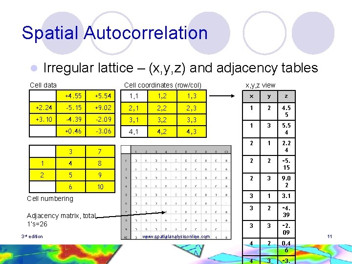
Spatial Autocorrelation Irregular lattice – (x, y, z) and adjacency tables l Cell data Cell coordinates (row/col) x, y, z view +4. 55 +5. 54 1, 1 1, 2 1, 3 x y z +2. 24 -5. 15 +9. 02 2, 1 2, 2 2, 3 1 2 +3. 10 -4. 39 -2. 09 3, 1 3, 2 3, 3 4. 5 5 +0. 46 -3. 06 4, 1 4, 2 4, 3 1 3 5. 5 4 2 1 2. 2 4 2 2 ‑ 5. 15 2 3 9. 0 2 3 1 3 2 ‑ 4. 39 3 3 ‑ 2. 09 3 7 1 4 8 2 5 9 6 10 Cell numbering Adjacency matrix, total 1’s=26 3 rd edition www. spatialanalysisonline. com 4 2 0. 4 6 4 3 ‑ 3. 11

Spatial Autocorrelation l “Spatial” (auto)correlation coefficient ¡ Coordinate (x, y, z) data representation for cells ¡ Spatial weights matrix (binary or other), W={wij} l From last slide: Σ wij=26 ¡ Coefficient formulation – desirable properties Reflects co-variation patterns l Reflects adjacency patterns via weights matrix l Normalised for absolute cell values l Normalised for data variation l Adjusts for number of included cells in totals l 3 rd edition www. spatialanalysisonline. com 12

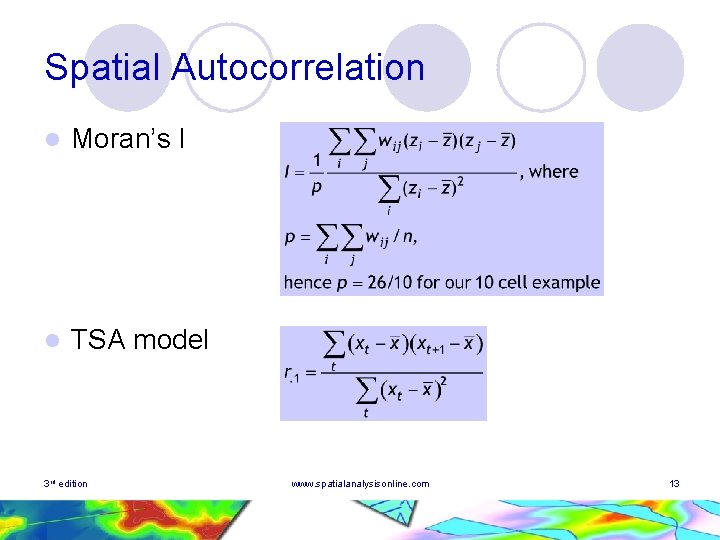
Spatial Autocorrelation l Moran’s I l TSA model 3 rd edition www. spatialanalysisonline. com 13

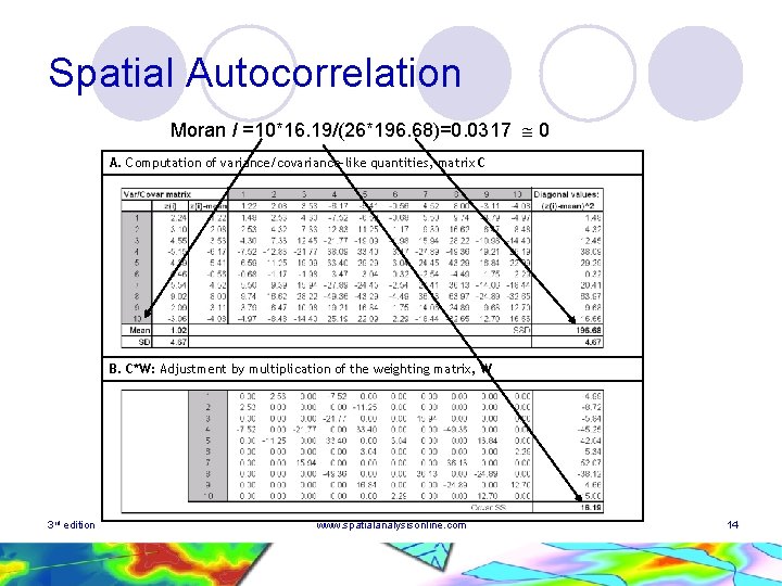
Spatial Autocorrelation Moran I =10*16. 19/(26*196. 68)=0. 0317 0 A. Computation of variance/covariance-like quantities, matrix C B. C*W: Adjustment by multiplication of the weighting matrix, W 3 rd edition www. spatialanalysisonline. com 14

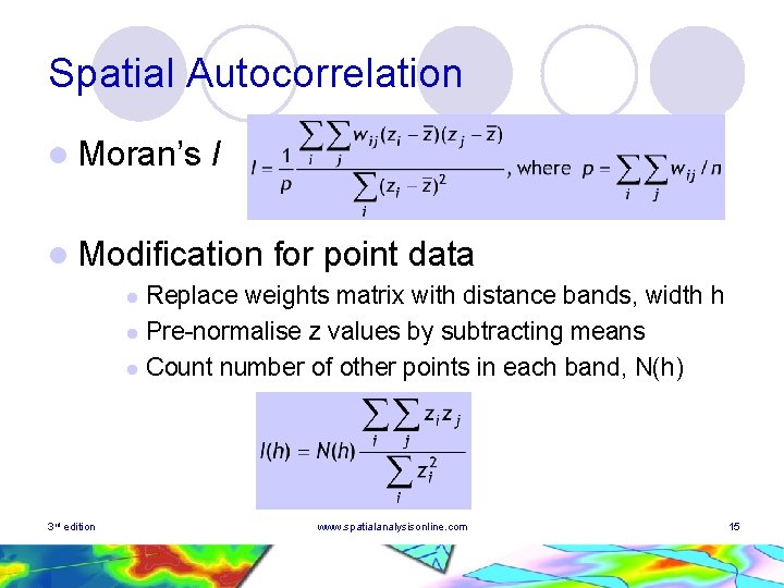
Spatial Autocorrelation l Moran’s I l Modification for point data Replace weights matrix with distance bands, width h l Pre-normalise z values by subtracting means l Count number of other points in each band, N(h) l 3 rd edition www. spatialanalysisonline. com 15

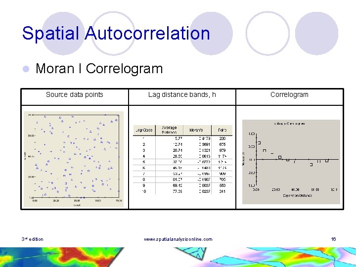
Spatial Autocorrelation l Moran I Correlogram Source data points 3 rd edition Lag distance bands, h www. spatialanalysisonline. com Correlogram 16

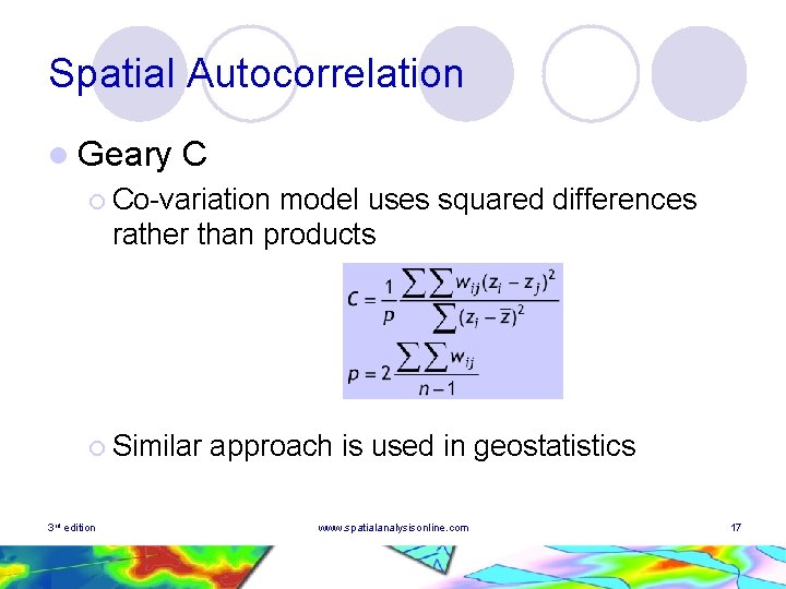
Spatial Autocorrelation l Geary C ¡ Co-variation model uses squared differences rather than products ¡ Similar 3 rd edition approach is used in geostatistics www. spatialanalysisonline. com 17

Spatial Autocorrelation l Extending SA concepts ¡ Distance formula weights vs bands ¡ Lattice models with more complex neighbourhoods and lag models (see Geo. Da) ¡ Disaggregation of SA index computations (rowwise) with/without row standardisation (LISA) ¡ Significance testing Normal model l Randomisation models l Bonferroni/other corrections l 3 rd edition www. spatialanalysisonline. com 18

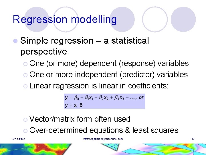
Regression modelling l Simple regression – a statistical perspective ¡ One (or more) dependent (response) variables ¡ One or more independent (predictor) variables ¡ Linear regression is linear in coefficients: ¡ Vector/matrix form often used ¡ Over-determined equations & least squares 3 rd edition www. spatialanalysisonline. com 19

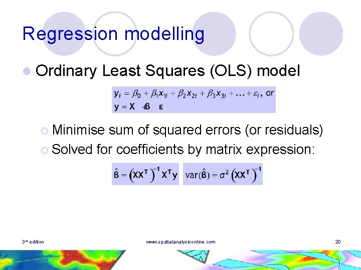
Regression modelling l Ordinary Least Squares (OLS) model ¡ Minimise sum of squared errors (or residuals) ¡ Solved for coefficients by matrix expression: 3 rd edition www. spatialanalysisonline. com 20

Regression modelling l OLS – models and assumptions ¡ Model – simplicity and parsimony ¡ Model – over-determination, multi-collinearity and variance inflation ¡ Typical assumptions Data are independent random samples from an underlying population l Model is valid and meaningful (in form and statistical) l Errors are iid l • Independent; No heteroskedasticity; common distribution l 3 rd edition Errors are distributed N(0, 2) www. spatialanalysisonline. com 21

Regression modelling l Spatial modelling and OLS ¡ Positive spatial autocorrelation is the norm, hence dependence between samples exists ¡ Datasets often non-Normal >> transformations may be required (Log, Box-Cox, Logistic) ¡ Samples are often clustered >> spatial declustering may be required ¡ Heteroskedasticity is common ¡ Spatial coordinates (x, y) may form part of the modelling process 3 rd edition www. spatialanalysisonline. com 22

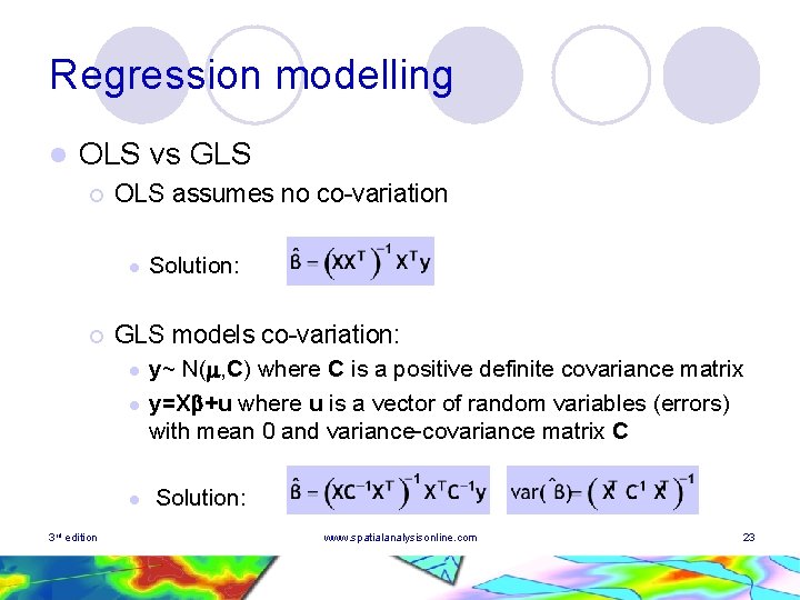
Regression modelling l OLS vs GLS ¡ OLS assumes no co-variation l ¡ GLS models co-variation: l l l 3 rd edition Solution: y~ N( , C) where C is a positive definite covariance matrix y=X +u where u is a vector of random variables (errors) with mean 0 and variance-covariance matrix C Solution: www. spatialanalysisonline. com 23

Regression modelling l GLS and spatial modelling ¡ ¡ l y~ N( , C) where C is a positive definite covariance matrix (C must be invertible) C may be modelled by inverse distance weighting, contiguity (zone) based weighting, explicit covariance modelling… Other models ¡ ¡ 3 rd edition Binary data – Logistic models Count data – Poisson models www. spatialanalysisonline. com 24

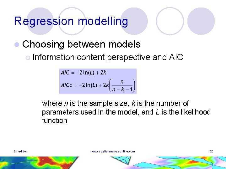
Regression modelling l Choosing between models ¡ Information content perspective and AIC where n is the sample size, k is the number of parameters used in the model, and L is the likelihood function 3 rd edition www. spatialanalysisonline. com 25

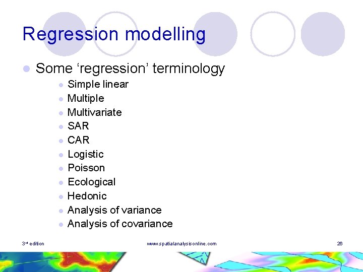
Regression modelling l Some ‘regression’ terminology l l l 3 rd edition Simple linear Multiple Multivariate SAR CAR Logistic Poisson Ecological Hedonic Analysis of variance Analysis of covariance www. spatialanalysisonline. com 26

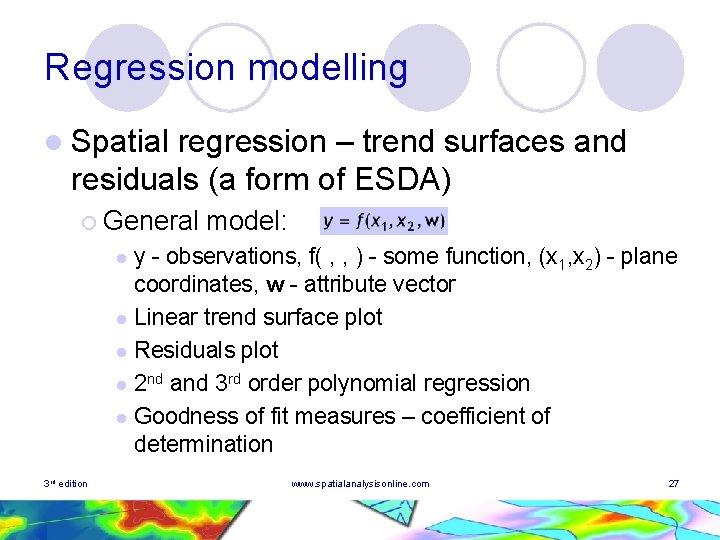
Regression modelling l Spatial regression – trend surfaces and residuals (a form of ESDA) ¡ General model: y - observations, f( , , ) - some function, (x 1, x 2) - plane coordinates, w - attribute vector l Linear trend surface plot l Residuals plot l 2 nd and 3 rd order polynomial regression l Goodness of fit measures – coefficient of determination l 3 rd edition www. spatialanalysisonline. com 27

Regression modelling l Regression & spatial autocorrelation (SA) ¡ Analyse the data for SA ¡ If SA ‘significant’ then Proceed and ignore SA, or l Permit the coefficient, , to vary spatially (GWR), or l Modify the regression model to incorporate the SA l 3 rd edition www. spatialanalysisonline. com 28

Regression modelling l Regression & spatial autocorrelation (SA) ¡ Analyse the data for SA ¡ If SA ‘significant’ then Proceed and ignore SA, or l Permit the coefficient, , to vary spatially (GWR) or l Modify the regression model to incorporate the SA l 3 rd edition www. spatialanalysisonline. com 29

Regression modelling l Geographically Weighted Regression (GWR) ¡ ¡ ¡ Coefficients, , allowed to vary spatially, (t) Model: Coefficients determined by examining neighbourhoods of points, t, using distance decay functions (fixed or adaptive bandwidths) Weighting matrix, W(t), defined for each point Solution: GLS: 3 rd edition www. spatialanalysisonline. com 30

Regression modelling l Geographically Weighted Regression ¡ Sensitivity – model, decay function, bandwidth, point/centroid selection ¡ ESDA – mapping of surface, residuals, parameters and SEs ¡ Significance testing Increased apparent explanation of variance l Effective number of parameters l AICc computations l 3 rd edition www. spatialanalysisonline. com 31

Regression modelling l Geographically ¡ Count Weighted Regression data – GWPR use of offsets l Fitting by ILSR methods l ¡ Presence/Absence data – GWLR True binary data l Computed binary data - use of re-coding, e. g. thresholding l Fitting by ILSR methods l 3 rd edition www. spatialanalysisonline. com 32

Regression modelling l Regression & spatial autocorrelation (SA) ¡ Analyse the data for SA ¡ If SA ‘significant’ then Proceed and ignore SA, or l Permit the coefficient, , to vary spatially (GWR) or l Modify the regression model to incorporate the SA l 3 rd edition www. spatialanalysisonline. com 33

Regression modelling l Regression & spatial autocorrelation (SA) ¡ Modify the regression model to incorporate the SA, i. e. produce a Spatial Autoregressive model (SAR) ¡ Many approaches – including: SAR – e. g. pure spatial lag model, mixed model, spatial error model etc. l CAR – a range of models that assume the expected value of the dependent variable is conditional on the (distance weighted) values of neighbouring points l Spatial filtering – e. g. OLS on spatially filtered data l 3 rd edition www. spatialanalysisonline. com 34

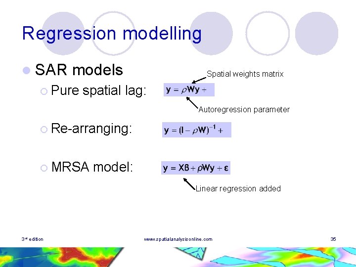
Regression modelling l SAR models ¡ Pure Spatial weights matrix spatial lag: Autoregression parameter ¡ Re-arranging: ¡ MRSA model: Linear regression added 3 rd edition www. spatialanalysisonline. com 35

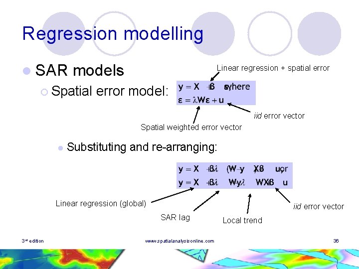
Regression modelling l SAR models ¡ Spatial Linear regression + spatial error model: iid error vector Spatial weighted error vector l Substituting and re-arranging: Linear regression (global) iid error vector SAR lag 3 rd edition www. spatialanalysisonline. com Local trend 36

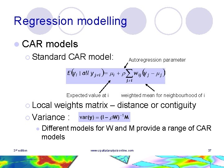
Regression modelling l CAR models ¡ Standard CAR model: Expected value at i Autoregression parameter weighted mean for neighbourhood of i ¡ Local weights matrix – distance or contiguity ¡ Variance : l 3 rd edition Different models for W and M provide a range of CAR models www. spatialanalysisonline. com 37

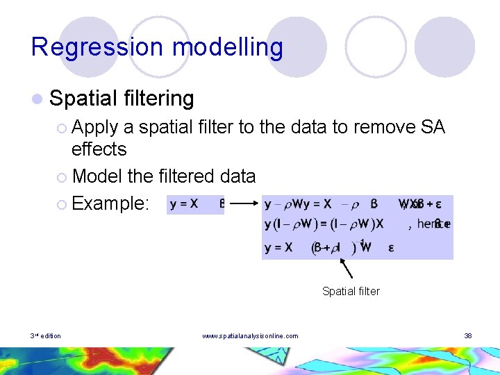
Regression modelling l Spatial filtering ¡ Apply a spatial filter to the data to remove SA effects ¡ Model the filtered data ¡ Example: Spatial filter 3 rd edition www. spatialanalysisonline. com 38