Chapter 5 OnLine Computer Control The z Transform

Chapter 5 On-Line Computer Control – The z Transform

Analysis of Discrete-Time Systems 1. The sampling process 2. z-transform 3. Properties of z-transforms 4. Analysis of open-loop and closed-loop discrete time systems 5. Design of discrete-time controllers

y Continuous signal Disontinuous y* signal y y* 9 1 3 5 7 9 11 1 t (sec) 3 6 t (sec) T = 1 sec y* (a) (b) 9 6 3 12 t (sec) T = 3 sec n y* (c) Continuous signal and its discrete-time representation with different sampling rates y* Dt t = n. T (a) y* t (b) t = n. T n Dt t = n. T t 12 t (c) From the response of a real sampler to the response of an ideal impulse sample

The Sampling Process y (t) 1. 2. Impulse Sampler y* At sampling times, strength of impulse is equal to value of input signal. Between sampling times, it is zero. Laplacing or

The Hold Process : From Discrete to Continuous Time discrete impulses m* (t) n Zero – Order Hold : n Transfer Function : Hold Device m (t) Continuous output Response of an impulse input : d (t) 1 m (t) m* (t) t T

First Order Hold Response to an impulse input 2 1 T 1 -1 Transfer function: 2 T

First Order versus Zero Order Hold m* (n. T) m (t) 0 1 T 3 T 5 T 7 T t 0 1 T 3 T 5 T (a) 7 T t (b) 0 1 T 3 T 5 T 7 T t (c) Comparison of reconstruction with zero-order and first-order holds, for slowly varying signals. m* (n. T) m (t) 0 2 T 4 T 6 T 8 T 10 T t 0 2 T 4 T 6 T 8 T (a) (b) 0 2 T 4 T 6 T 8 T 10 T t (c) Comparison of reconstruction with zero-order and first-order holds, for rapidly changing signals. 10 T t

Z-Transforms y(t) Sample yz(t) Remarks 1. z-transform depends only on the discrete values y(0), y( )ז. . etc. If two continuous functions have the sampled values , then ztransform will be the same. 2. It is assumed that the summation exists and is finit. 3. We can also view t in the form Z[ y (s) ] = ŷ(z)

Z-Transforms of Basic Functions 1. Unit Step Function 2. Exponential Function

Z-Transforms of Basic Functions Continued 3. Ramp Function 4. Trigonometric Functions

Z-Transforms of Basic Functions Continued 5. Translation

Z-transform for Numerical Derivative z-1 is like a back shift operator

Properties of z-Transforms 1. Linearity 2. Final Value Theorem

Numerical Integration in z-transform Using Trapezoidal Rule or solving

Inversion of z-transforms 1. Partial fraction expansion λ 1, λ 2, … λn are low-order polynomials in z-1 compute c 1, c 2, …cn. Invert each part separately, we able

From Tables of z-transforms y(n. T) = -1/2 + 1/2 e 11 n y: 0, 1, 4, 13, 0, … 2. Inversion by Long-Division 1 -4 z-1+3 z-2 y(0) = 0 y(T) = 1 y(2 T) = 4 y(3 T) = 13 1 z-1+4 z-2+13 z-3 z-1 -4 z-2+3 z-3 4 z-2 -16 z-3+12 z-4 13 z-3 -12 z-4

z-transforms of various functions Function in time domain Lalpace transform unit impluse 1 unit step 1/s ramp: f(t) = at a/s 2 f(t) = tn n!/sn+1 f(t) = e-at 1/s+a f(t) =te-at 1/(s+a)2 z-transform

z-transforms of various functions Function in time domain f(t) = sinωt f(t) = cosωt f(t) = 1 -e-at f(t) = e-at sinωt f(t) = e-at cosωt Lalpace transform z-transform

Discrete-Time Response of systems In computer control: measurements are taken periodically and control actions implemented periodically, This results in a discrete input/discrete output dynamic system. cn en Discrete System

Example of Discrete Systems Let a discrete time approximation is Taking z-transform

Z-transform for a given continuous system with transfer function G(s) and a ZOH

Example: Pure Integrator with Hold c*(s) Step response Hence of which impulse a ramp response y*(s )

Example：First order lag system

Step Response for 1 st order lag system From tables, for y(t) ＊ ＊ ＊ time Note: Compare with discrete approximation to First-order system

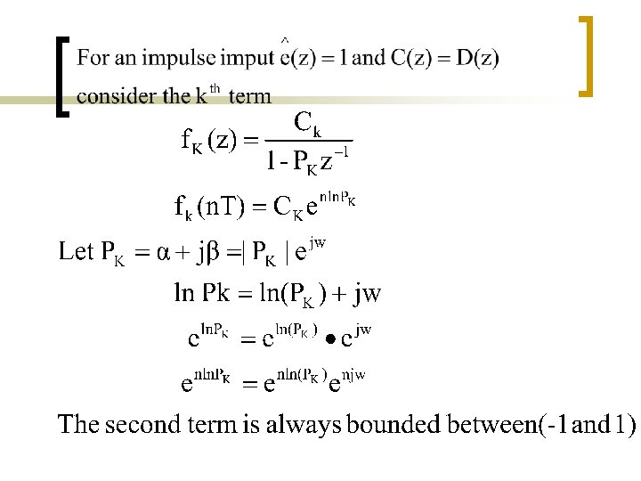
Generalization or D (z)=Transfer function relating e and c Analogous to Laplace transfer Discrete time input/output model Remark： Note that D(z) is the z-transform of the response of the system to an impulse input

Z-transform of a continuous process with Sample and Hold H (s) discrete input Process Gp (s) c*(s) y (s) continuous variables y*(s) discrete output we seek a relationship (Z-transfer function) between c and y. Consider a impulse input c*(z)=1 c*(s)=1 Then HGp(z) called the pulse transfer function (since it represents the z-transform of the pulse response of Gp (s) )

Properties of pulse Transfer Function 1. 2. An impulse input is converted into a pulse input by the first order hold element. Hence HG(z) is the pulse response of G(s) sampled at z internals of T. 3. The pulse transfer function of two systems in series can be combined if there is a sample and hold in between. c 2 c 1 T G 1(z) G 2(z) c 3

Closed-Loop System T set point + ysp (z) D (z) T Hold Process H (s) Gp (s) m (s) - disturbance sampled output or 1. Roots of the Characteristic equation 1+HGp(z)D(z)=0 Determine stability of the closed-loop system 2. Note similarity to continuous system. y(2) y 1(s)

Example: closed-loop response of a first-order system For proportional control where

For a unit step change in set point and

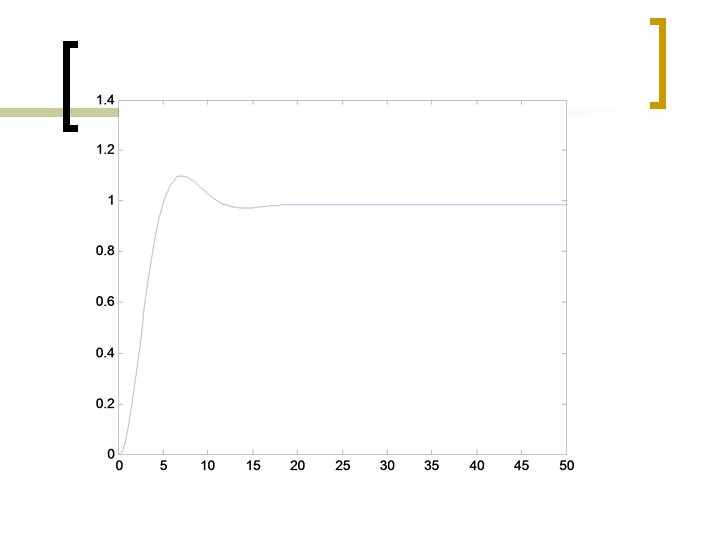
n The response is very similar to continuous control. The steady state value of y(t) is Hence the offset is

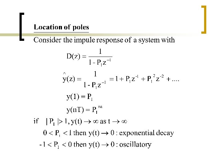
Stability of Discrete Systems A system is consider to be stable if output remains bounded for bounded Inputs. Consider a discrete system with transfer function Where P 1, P 2, …, Pn are n roots of:

Im Unstable roots real STABLE REGION Unit circle

Example: Stability of closed-loop

Example: Stability of closedloop - Continued

Digital Feedback - Control

n 1. 2. 3. n No initialization is necessary. [ Cs is not needed ] Bumpless transfer from manual / automatic Automatic ‘reset-windup’ protection. Protection in case of computer failure Disadvantages: 1. 2. n Advantages of velocity Form Since different modes are indistinguishable, on-line tuning methods will not work. Difficult to put constraints on integral and / or derivative term. Tuning Digital Controllers: 1. 2. 3. Ziegler – Nichols Cohen – Coon settings Time - integral performance criteria

Y(t) actual ideal time

Derivation of Deadbeat Controller- Continued

Deadbeat

Deadbeat 0~10 sec

Deadbeat control for (1/(s+1)3) n Sampling time: 2

Ringing and Pole-placement Ringing refers to excessive value movement caused by a widely oscillating controller output. Caused by negative poles in D(z). Hence avoid poles near -1. Change controller design such that poles are on the side or near zero on negative side

n SYS = TF(1, [1 3 3 1]) n n n Transfer function: 1 ----------s^3 + 3 s^2 + 3 s + 1 n n >> sysd=c 2 d(SYS, 2) n n n Transfer function: 0. 3233 z^2 + 0. 3073 z + 0. 01584 -------------------z^3 - 0. 406 z^2 + 0. 05495 z - 0. 002479 n n Sampling time: 2 0. 3233 0. 6306 0. 3231 n >> p 1=[1 -1]; p 2=[0. 3233 0. 3073 0. 01584] n p 2 = n n 0. 3233 0. 3073 n >> c=conv(p 1, p 2) n c= n 0. 0158 0. 3233 -0. 0160 -0. 2915 -0. 0158

Canceling the ringing pole at z=-0. 8958 n n ans = 1. 0000 -0. 8958 -0. 0547 n >> p 1=[1 0]; p 2=[1 -0. 99]; p 3=[1 0. 0547]; >> c=conv(p 1, p 2) n c= n n 1. 0000 -0. 9900 n >> c=conv(c, p 3) n c= n n n 0 1. 0000 -0. 9353 -0. 0542 0 Warning: Using a default value of 1 for maximum step size. The simulation step size will be limited to be less than this value. >>

Smoothing the Control Action n n n p=[0. 3233 -0. 016 -0. 2915 -0. 01584]; r=roots(p) r= 1. 0001 -0. 8959 -0. 0547 Delete the unstable pole z=-0. 8959 n p 1=[1 -0. 99]; p 2=[1 0. 0547]; c=conv(p 1, p 2) n c= n n 1. 0000 -0. 9353 -0. 0542

Reconstruct the Control Loop

The treatment of unstable poles n sysd=c 2 d(SYS, 1) n n n Transfer function: 0. 0803 z^2 + 0. 1544 z + 0. 01788 -----------------z^3 - 1. 104 z^2 + 0. 406 z - 0. 04979 n n >> p 2=[ 0. 0803 0. 1544 0. 01788] n p 2 = n 0. 0803 0. 1544 n >> p 1=[1 -1] n p 1 = n 1 -1 n >> c=conv(p 1, p 2) n c= n 0. 0179 0. 0803 0. 0741 -0. 1365 -0. 0179

The treatment of unstable poles n >> roots(c) n ans = n n n -1. 7990 1. 0000 -0. 1238 n >> p 1=[1 0]; p 2=[1 -0. 99]; p 3=[1 0. 1238]; >> c=conv(p 1, p 2) n c= n n 1. 0000 -0. 9900 n >> c=conv(c, p 3) n c= n 0 1. 0000 -0. 8662 -0. 1226 0

3. Dahlin’s Method n Require that the closed–loop system behave like a first-order system with dead-time. we want for Solving for D 1. Choose m, q such that D(z) is realizable 2. Lot of algebra

Dahlin’s Method

Dahlin’s Method 0~10 sec 0~50 sec

Dahlin’s Method for (1/(s+1)3) n Sampling time: 2

Regulatory Control Consider a process described by yn = a 1 yn-1 + a 2 yn-2 + … + b 1 mn-1 + … + bk mn-k In regulatory control, we want to keep y close to zero in presence of disturbances. Ideally choose mn such that yn ≡ ysp è ysp = a 1 yn + a 2 yn-2 + … + bkyn-k+1 + b 1 mn + b 2 mn-1 + bkmn-k+1 Or mn = -1/b 1 [ ysp – a 1 yn – a yn-1 - akyn-k+1 – b 2 mn-1 + … - bkmn-k+1 ] Remark 1. Problems can arise in practice if model parameters are not known 2. The above choice is equivalent to minimizing 3. If dead-time is present control will be unrealizable