Chapter 5 Normal Probability Distributions Section 5 4

Chapter 5 Normal Probability Distributions Section 5 -4 – Sampling Distributions and the Central Limit Theorem A. A sampling distribution is the probability distribution of a sample statistic that is formed when samples of size n are repeatedly taken from a population. 1. If the sample statistic is the sample mean, then the distribution is the sampling distribution of sample means. a. Every sample statistic has a sampling distribution. 2. Remember that sample means can vary from one another and can also vary from the population mean. a. This type of variation is to be expected and is called sampling error. 3. Properties of sampling distributions of sample means: a. The mean of the sample means is equal to the population mean.

Chapter 5 Normal Probability Distributions Section 5 -4 – Sampling Distributions and the Central Limit Theorem b. The standard deviation of the sample means is equal to the population standard deviation divided by the square root of n. 1) The standard deviation of the sampling distribution of the sample means is called the standard error of the mean. B. The Central Limit Theorem 1. The Central Limit Theorem forms the foundation for the inferential branch of statistics. a. It describes the relationship between the sampling distribution of sample means and the population that the samples are taken from. b. It is an important tool that provides the information you’ll need to use sample statistics to make inferences about a population mean.

Chapter 5 Normal Probability Distributions Section 5 -4 – Sampling Distributions and the Central Limit Theorem 2. The Central Limit Theorem says: a. If samples of size n, where n ≥ 30, are drawn from any population with a mean μ and a standard deviation σ, then the sampling distribution of sample means approximates a normal distribution. 1) The greater the sample size (the larger number n is), the better the approximation. b. If the population itself is normally distributed, the sampling distribution of sample means is normally distributed for any sample size n. 3. Whether the original population distribution is normal or not, the sampling distribution of sample means has a mean equal to the population mean.

Chapter 5 Normal Probability Distributions Section 5 -4 – Sampling Distributions and the Central Limit Theorem a. In real life words, this means that if we take the average of all of the means, from all of the samples that are done on one population, the mean of those averages will equal the mean of the population. 4. The sampling distribution of sample means has a variance equal to 1/n times the variance of the population. a. The standard deviation of sample means will be smaller than the standard deviation of the population. 5. The sampling distribution of sample means has a standard deviation equal to the population standard deviation divided by the square root of n. a. The distribution of sample means has the same center as the population, but it is not as spread out.

Chapter 5 Normal Probability Distributions Section 5 -4 – Sampling Distributions and the Central Limit Theorem 1) The bigger n (the sample size) gets, the smaller the standard deviation will get. a) The more times we take a sample of the same population, the more tightly grouped the results will be. b. The standard deviation of the sampling distribution of the sample means, σₓ, is also called the standard error of the mean. C. Probability and the Central Limit Theorem 1. Using what we’ve learned in Section 5 -2, and what we’ve been told here in Section 5 -4, we can find the probability that a sample mean will fall in a given interval of the sampling distribution.

Chapter 5 Normal Probability Distributions Section 5 -4 – Sampling Distributions and the Central Limit Theorem a. To find a z-score of a random variable x, we took the value minus the mean and divided by the standard deviation. b. To convert the sample mean to a z-score, we alter that slightly. 1) Instead of dividing by the standard deviation, we divide by the sample error. a) Remember, this is the standard deviation of the population divided by the square root of n (the sample size).

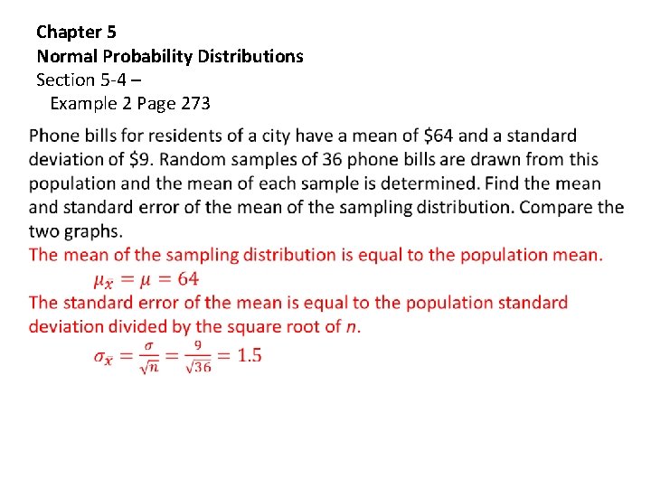
Chapter 5 Normal Probability Distributions Section 5 -4 – Example 2 Page 273

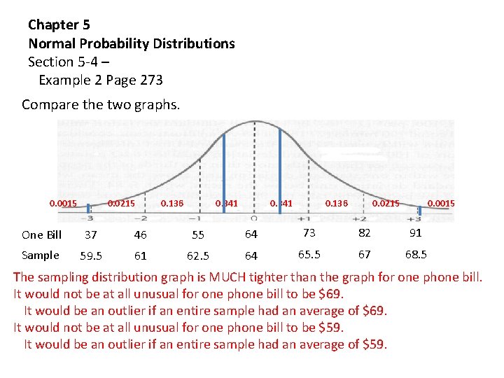
Chapter 5 Normal Probability Distributions Section 5 -4 – Example 2 Page 273 Compare the two graphs. 0. 0015 0. 0215 0. 136 0. 341 0. 136 0. 0215 0. 0015 One Bill 37 46 55 64 73 82 91 Sample 59. 5 61 62. 5 64 65. 5 67 68. 5 The sampling distribution graph is MUCH tighter than the graph for one phone bill. It would not be at all unusual for one phone bill to be $69. It would be an outlier if an entire sample had an average of $69. It would not be at all unusual for one phone bill to be $59. It would be an outlier if an entire sample had an average of $59.

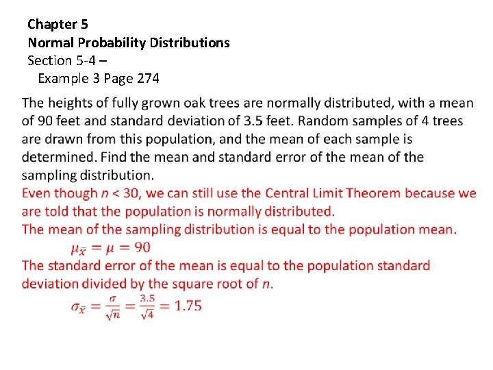
Chapter 5 Normal Probability Distributions Section 5 -4 – Example 3 Page 274

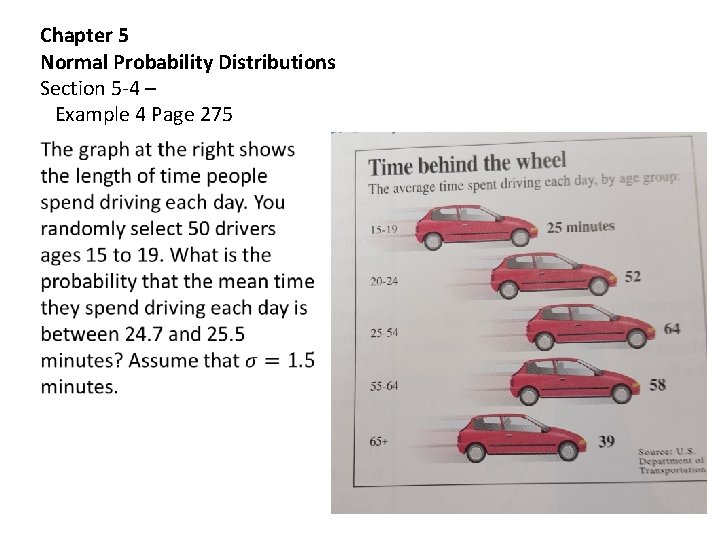
Chapter 5 Normal Probability Distributions Section 5 -4 – Example 4 Page 275

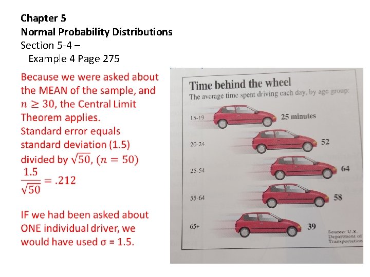
Chapter 5 Normal Probability Distributions Section 5 -4 – Example 4 Page 275

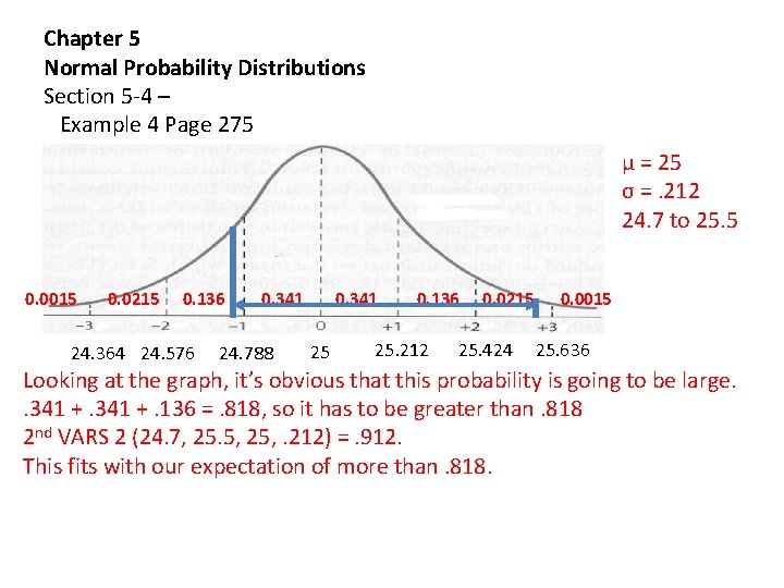
Chapter 5 Normal Probability Distributions Section 5 -4 – Example 4 Page 275 µ = 25 σ =. 212 24. 7 to 25. 5 0. 0015 0. 0215 0. 136 24. 364 24. 576 0. 341 24. 788 0. 341 25 0. 136 25. 212 0. 0215 25. 424 0. 0015 25. 636 Looking at the graph, it’s obvious that this probability is going to be large. . 341 +. 136 =. 818, so it has to be greater than. 818 2 nd VARS 2 (24. 7, 25. 5, 25, . 212) =. 912. This fits with our expectation of more than. 818.

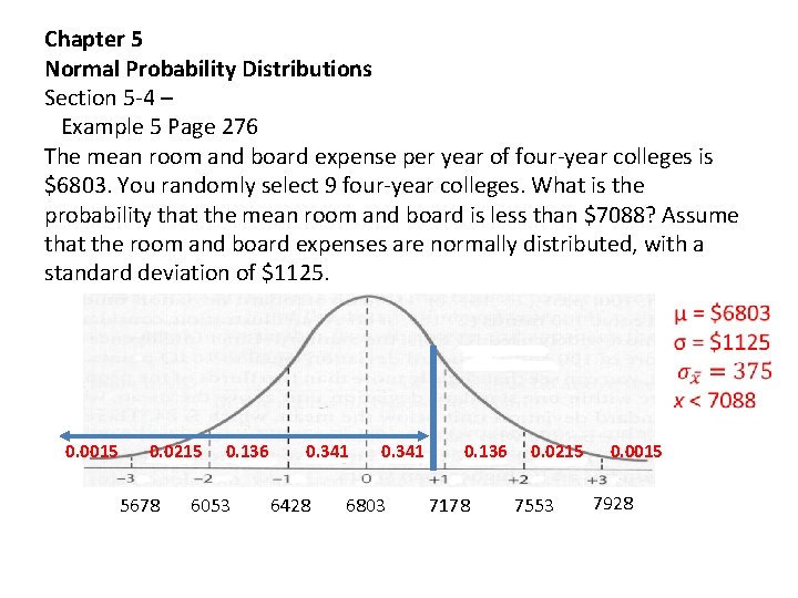
Chapter 5 Normal Probability Distributions Section 5 -4 – Example 5 Page 276 The mean room and board expense per year of four-year colleges is $6803. You randomly select 9 four-year colleges. What is the probability that the mean room and board is less than $7088? Assume that the room and board expenses are normally distributed, with a standard deviation of $1125. 0. 0015 0. 0215 5678 0. 136 6053 0. 341 6428 0. 341 6803 0. 136 7178 0. 0215 7553 0. 0015 7928

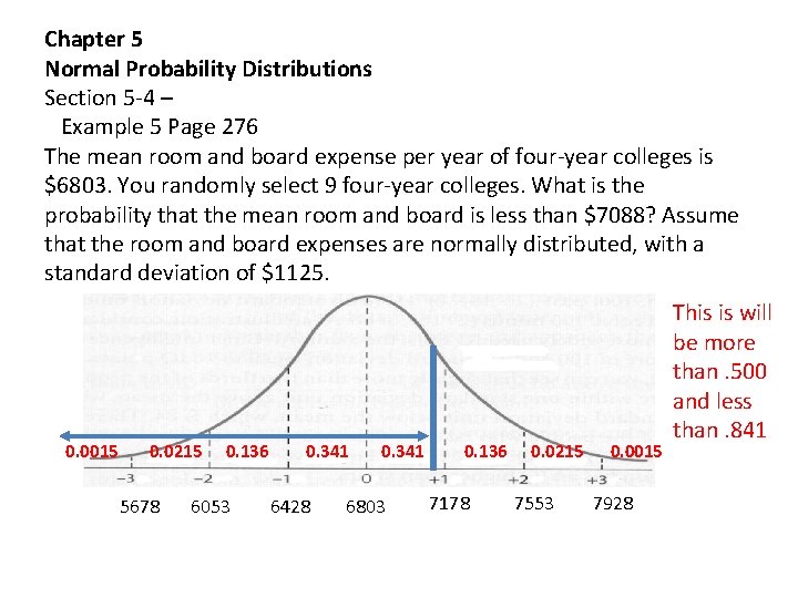
Chapter 5 Normal Probability Distributions Section 5 -4 – Example 5 Page 276 The mean room and board expense per year of four-year colleges is $6803. You randomly select 9 four-year colleges. What is the probability that the mean room and board is less than $7088? Assume that the room and board expenses are normally distributed, with a standard deviation of $1125. 0. 0015 0. 0215 5678 0. 136 6053 0. 341 6428 0. 341 6803 0. 136 7178 0. 0215 7553 0. 0015 7928 This is will be more than. 500 and less than. 841

Chapter 5 Normal Probability Distributions Section 5 -4 – Example 5 Page 276 The mean room and board expense per year of four-year colleges is $6803. You randomly select 9 four-year colleges. What is the probability that the mean room and board is less than $7088? Assume that the room and board expenses are normally distributed, with a standard deviation of $1125. 2 nd VARS 2 (-1 E 99, 7088, 6803, 375) =. 776 This is in line with our guess of more than. 500 and less than. 841. ALSO, 2 nd VARS 3 (. 776, 6803, 375) = 7087. 533, which confirms our answer. So, you have a. 776 probability of paying less than $7088 for room and board.

Chapter 5 Normal Probability Distributions Section 5 -4 – Example 6 Page 277 A bank auditor claims that credit card balances are normally distributed, with a mean of $2870 and a standard deviation of $900. 1) What is the probability that a randomly selected credit card holder has a credit card balance less than $2500? 2) You randomly select 25 credit card holders. What is the probability that their mean credit card balance is less than $2500? 3) Compare the probabilities from (1) and (2) and interpret your answer in terms of the auditor’s claim.

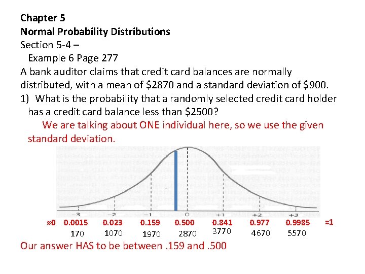
Chapter 5 Normal Probability Distributions Section 5 -4 – Example 6 Page 277 A bank auditor claims that credit card balances are normally distributed, with a mean of $2870 and a standard deviation of $900. 1) What is the probability that a randomly selected credit card holder has a credit card balance less than $2500? We are talking about ONE individual here, so we use the given standard deviation. ≈0 0. 0015 170 0. 023 1070 0. 159 1970 0. 500 2870 0. 841 3770 Our answer HAS to be between. 159 and. 500 0. 977 4670 0. 9985 5570 ≈1

Chapter 5 Normal Probability Distributions Section 5 -4 – Example 6 Page 277 A bank auditor claims that credit card balances are normally distributed, with a mean of $2870 and a standard deviation of $900. 1) What is the probability that a randomly selected credit card holder has a credit card balance less than $2500? 2 nd VARS 2 (-1 E 99, 2500, 2870, 900) =. 340 This fits our estimate of between. 159 and. 500 We can also check this with the inv. Norm function. 2 nd VARS 3 (. 340, 2870, 900) = 2498. 78 Our answer checks.

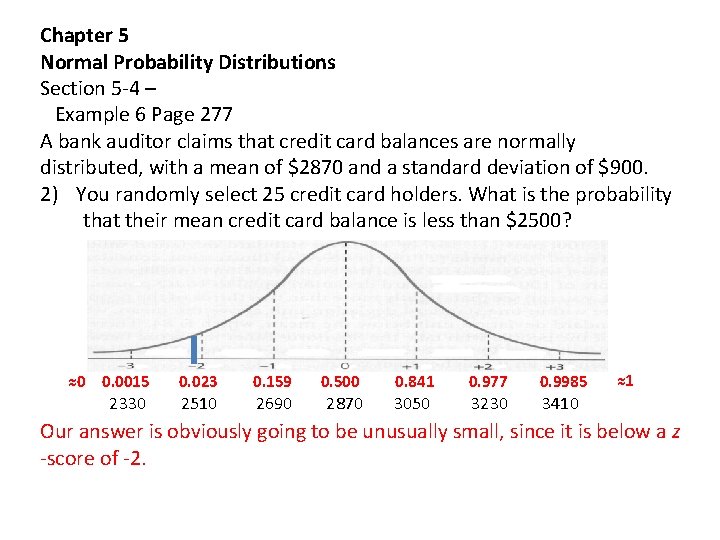
Chapter 5 Normal Probability Distributions Section 5 -4 – Example 6 Page 277 A bank auditor claims that credit card balances are normally distributed, with a mean of $2870 and a standard deviation of $900. 2) You randomly select 25 credit card holders. What is the probability that their mean credit card balance is less than $2500? ≈0 0. 0015 0. 023 0. 159 0. 500 0. 841 0. 977 0. 9985 2330 2510 2690 2870 3050 3230 3410 ≈1 Our answer is obviously going to be unusually small, since it is below a z -score of -2.

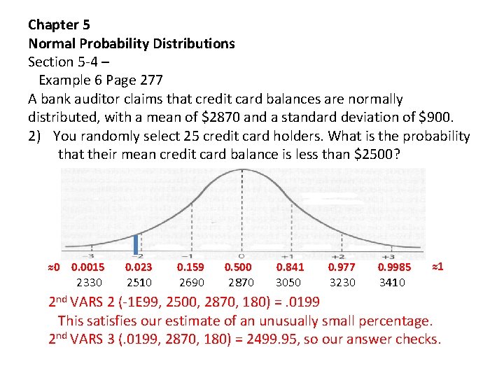
Chapter 5 Normal Probability Distributions Section 5 -4 – Example 6 Page 277 A bank auditor claims that credit card balances are normally distributed, with a mean of $2870 and a standard deviation of $900. 2) You randomly select 25 credit card holders. What is the probability that their mean credit card balance is less than $2500? ≈0 0. 0015 0. 023 0. 159 0. 500 0. 841 0. 977 0. 9985 2330 2510 2690 2870 3050 3230 3410 ≈1 2 nd VARS 2 (-1 E 99, 2500, 2870, 180) =. 0199 This satisfies our estimate of an unusually small percentage. 2 nd VARS 3 (. 0199, 2870, 180) = 2499. 95, so our answer checks.

Chapter 5 Normal Probability Distributions Section 5 -4 – Example 6 Page 277 A bank auditor claims that credit card balances are normally distributed, with a mean of $2870 and a standard deviation of $900. 3) Compare the probabilities from (1) and (2) and interpret your answer in terms of the auditor’s claim. The probability of a single card holder owing less than $2500 is 34%, but the probability that the average of 25 card holders balances is less than $2500 is less than 2%. Remember, less than 2% is considered to be unusual. Either the auditor is wrong about the distribution being normal, or your sample is unusual and needs to be done again, more carefully.

Your Assignments are: Classwork: Pages 278– 279, #1– 8, 11– 16 All Homework: Pages 279– 282, #18– 38 Evens You do not need to turn in the graph sketches.