Chapter 5 Normal Distribution 5 1 5 2

Chapter 5. Normal Distribution 5. 1 5. 2 5. 3 5. 4 NIPRL Probability Calculation Using the Normal Distribution Linear Combinations of Normal Random Variables Approximating Distributions with the Normal Distributions Related to the Normal Distribution

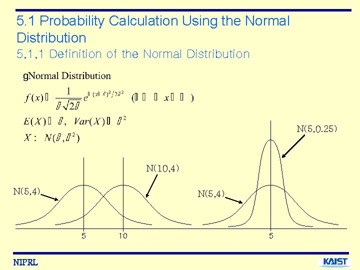
5. 1 Probability Calculation Using the Normal Distribution 5. 1. 1 Definition of the Normal Distribution N(5, 0. 25) N(10, 4) N(5, 4) 5 NIPRL 10 5

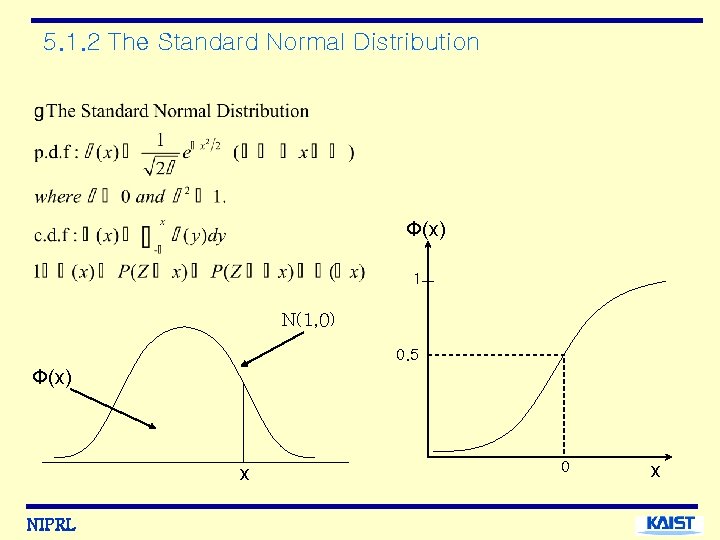
5. 1. 2 The Standard Normal Distribution Ф(x) 1 N(1, 0) 0. 5 Ф(x) x NIPRL 0 x

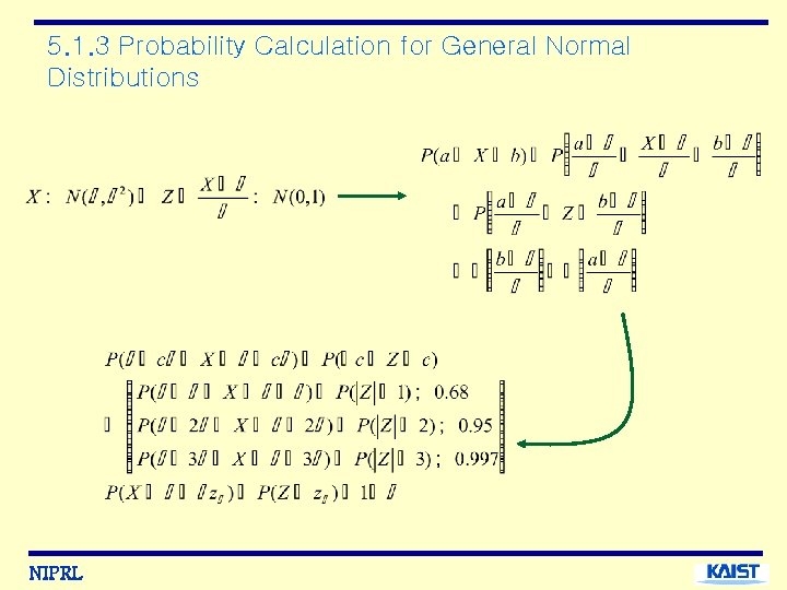
5. 1. 3 Probability Calculation for General Normal Distributions NIPRL

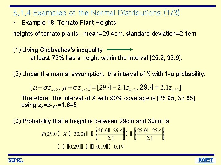
5. 1. 4 Examples of the Normal Distributions (1/3) • Example 18: Tomato Plant Heights heights of tomato plants : mean=29. 4 cm, standard deviation=2. 1 cm (1) Using Chebychev’s inequality at least 75% has a height within the interval [25. 2, 33. 6]. (2) Under the normal assumption, the interval of X with 1 -α probability: Therefore, the interval of X with 90% coverage is [25. 95, 32. 85] using zα=z 0. 05=1. 645 (3) Probability that a height is between 29 cm and 30 cm is NIPRL

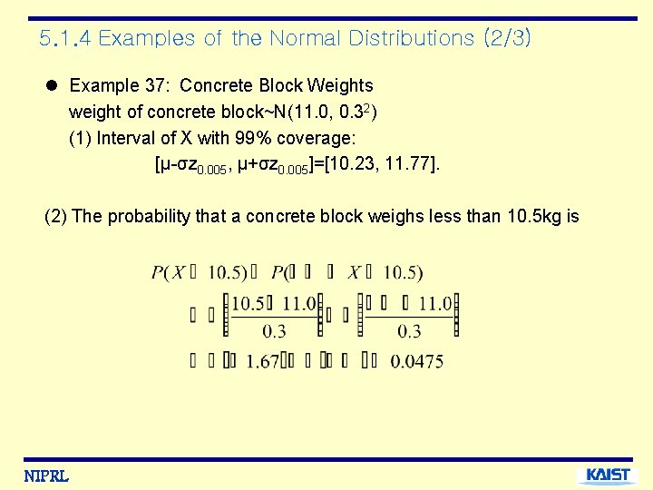
5. 1. 4 Examples of the Normal Distributions (2/3) l Example 37: Concrete Block Weights weight of concrete block~N(11. 0, 0. 32) (1) Interval of X with 99% coverage: [μ-σz 0. 005, μ+σz 0. 005]=[10. 23, 11. 77]. (2) The probability that a concrete block weighs less than 10. 5 kg is NIPRL

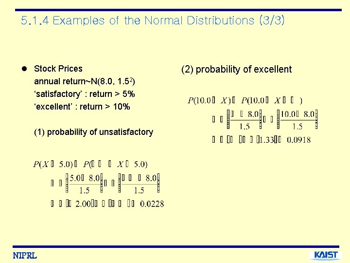
5. 1. 4 Examples of the Normal Distributions (3/3) l Stock Prices annual return~N(8. 0, 1. 52) ‘satisfactory’ : return > 5% ‘excellent’ : return > 10% (1) probability of unsatisfactory NIPRL (2) probability of excellent

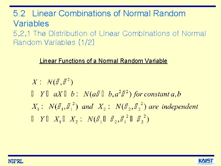
5. 2 Linear Combinations of Normal Random Variables 5. 2. 1 The Distribution of Linear Combinations of Normal Random Variables (1/2) Linear Functions of a Normal Random Variable NIPRL

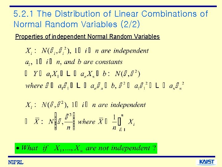
5. 2. 1 The Distribution of Linear Combinations of Normal Random Variables (2/2) Properties of independent Normal Random Variables NIPRL

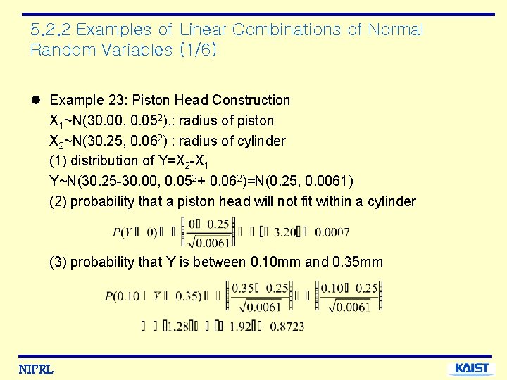
5. 2. 2 Examples of Linear Combinations of Normal Random Variables (1/6) l Example 23: Piston Head Construction X 1~N(30. 00, 0. 052), : radius of piston X 2~N(30. 25, 0. 062) : radius of cylinder (1) distribution of Y=X 2 -X 1 Y~N(30. 25 -30. 00, 0. 052+ 0. 062)=N(0. 25, 0. 0061) (2) probability that a piston head will not fit within a cylinder (3) probability that Y is between 0. 10 mm and 0. 35 mm NIPRL

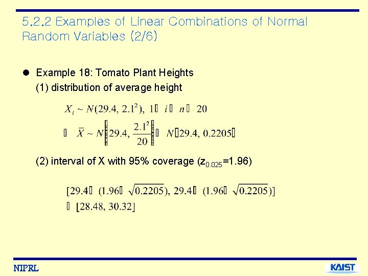
5. 2. 2 Examples of Linear Combinations of Normal Random Variables (2/6) l Example 18: Tomato Plant Heights (1) distribution of average height (2) interval of X with 95% coverage (z 0. 025=1. 96) NIPRL

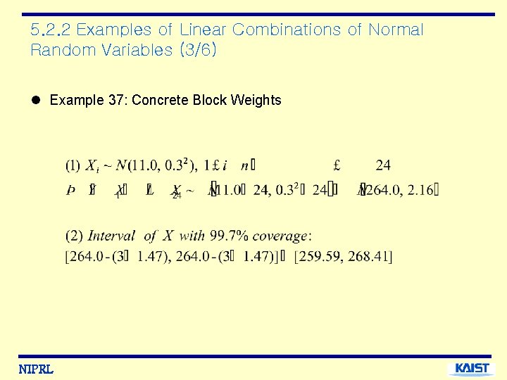
5. 2. 2 Examples of Linear Combinations of Normal Random Variables (3/6) l Example 37: Concrete Block Weights NIPRL

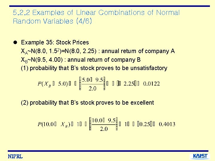
5. 2. 2 Examples of Linear Combinations of Normal Random Variables (4/6) l Example 35: Stock Prices XA~N(8. 0, 1. 52)=N(8. 0, 2. 25) : annual return of company A XB~N(9. 5, 4. 00) : annual return of company B (1) probability that B’s stock proves to be unsatisfactory (2) probability that B’s stock proves to be excellent NIPRL

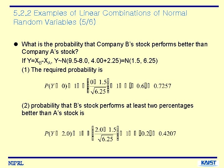
5. 2. 2 Examples of Linear Combinations of Normal Random Variables (5/6) l What is the probability that Company B’s stock performs better than Company A’s stock? If Y=XB-XA, Y~N(9. 5 -8. 0, 4. 00+2. 25)=N(1. 5, 6. 25) (1) The required probability is (2) probability that B’s stock performs at least two percentages better than A’s stock is NIPRL

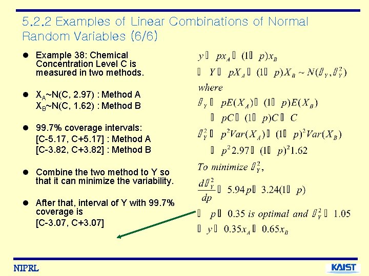
5. 2. 2 Examples of Linear Combinations of Normal Random Variables (6/6) l Example 38: Chemical Concentration Level C is measured in two methods. l XA~N(C, 2. 97) : Method A XB~N(C, 1. 62) : Method B l 99. 7% coverage intervals: [C-5. 17, C+5. 17] : Method A [C-3. 82, C+3. 82] : Method B l Combine the two method to Y so that it can minimize the variability. l After that, interval of Y with 99. 7% coverage is [C-3. 07, C+3. 07] NIPRL

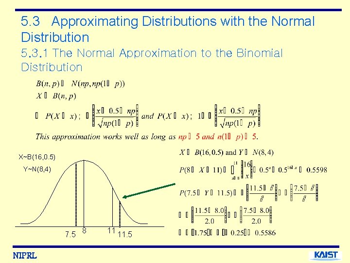
5. 3 Approximating Distributions with the Normal Distribution 5. 3. 1 The Normal Approximation to the Binomial Distribution X~B(16, 0. 5) Y~N(8, 4) 7. 5 NIPRL 8 11 11. 5

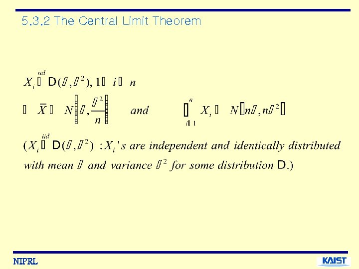
5. 3. 2 The Central Limit Theorem NIPRL

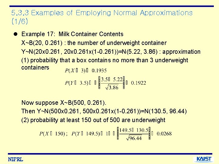
5. 3. 3 Examples of Employing Normal Approximations (1/6) l Example 17: Milk Container Contents X~B(20, 0. 261) : the number of underweight container Y~N(20 x 0. 261, 20 x 0. 261 x(1 -0. 261))=N(5. 22, 3. 86) : approximation (1) probability that a box contains no more than 3 underweight containers Now suppose X~B(500, 0. 261). Then Y~N(500 x 0. 261, 500 x 0. 261 x(1 -0. 261))=N(130. 5, 96. 44) (2) probability at least 150 out of 500 are underweight NIPRL

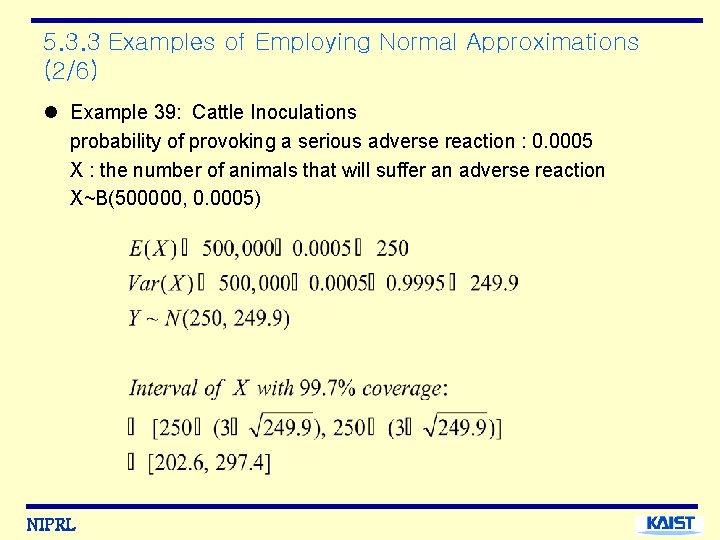
5. 3. 3 Examples of Employing Normal Approximations (2/6) l Example 39: Cattle Inoculations probability of provoking a serious adverse reaction : 0. 0005 X : the number of animals that will suffer an adverse reaction X~B(500000, 0. 0005) NIPRL

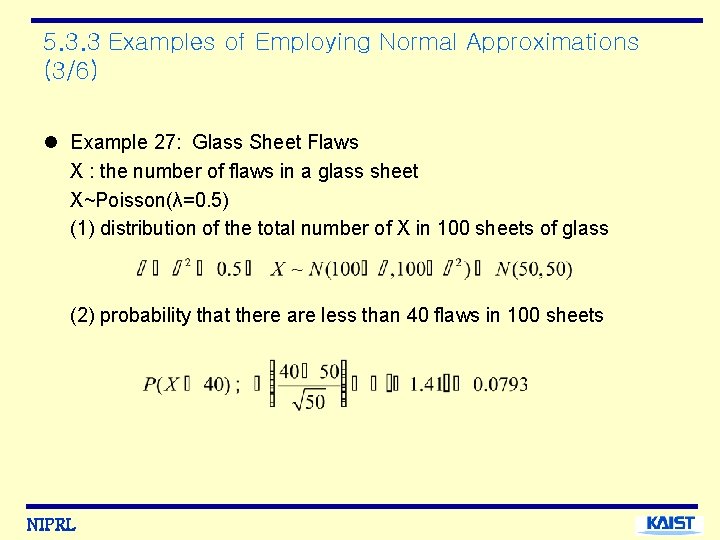
5. 3. 3 Examples of Employing Normal Approximations (3/6) l Example 27: Glass Sheet Flaws X : the number of flaws in a glass sheet X~Poisson(λ=0. 5) (1) distribution of the total number of X in 100 sheets of glass (2) probability that there are less than 40 flaws in 100 sheets NIPRL

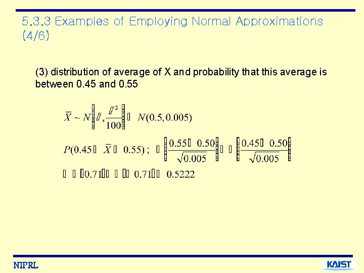
5. 3. 3 Examples of Employing Normal Approximations (4/6) (3) distribution of average of X and probability that this average is between 0. 45 and 0. 55 NIPRL

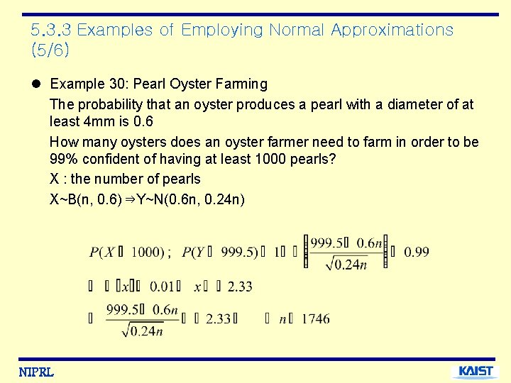
5. 3. 3 Examples of Employing Normal Approximations (5/6) l Example 30: Pearl Oyster Farming The probability that an oyster produces a pearl with a diameter of at least 4 mm is 0. 6 How many oysters does an oyster farmer need to farm in order to be 99% confident of having at least 1000 pearls? X : the number of pearls X~B(n, 0. 6)⇒Y~N(0. 6 n, 0. 24 n) NIPRL

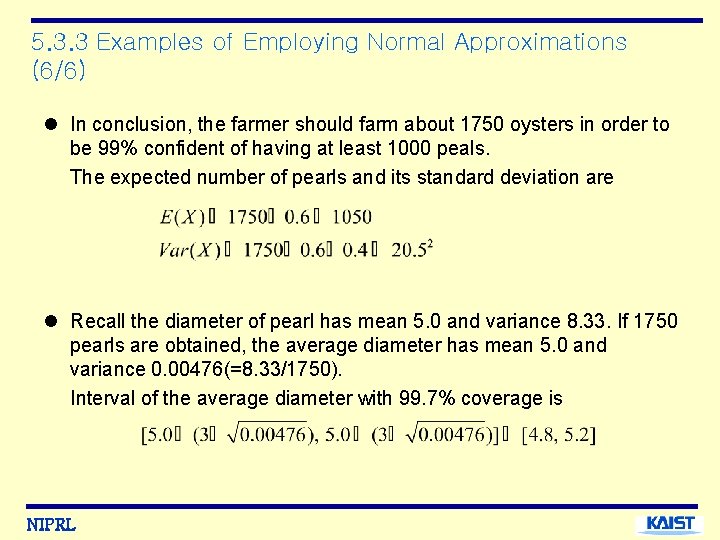
5. 3. 3 Examples of Employing Normal Approximations (6/6) l In conclusion, the farmer should farm about 1750 oysters in order to be 99% confident of having at least 1000 peals. The expected number of pearls and its standard deviation are l Recall the diameter of pearl has mean 5. 0 and variance 8. 33. If 1750 pearls are obtained, the average diameter has mean 5. 0 and variance 0. 00476(=8. 33/1750). Interval of the average diameter with 99. 7% coverage is NIPRL

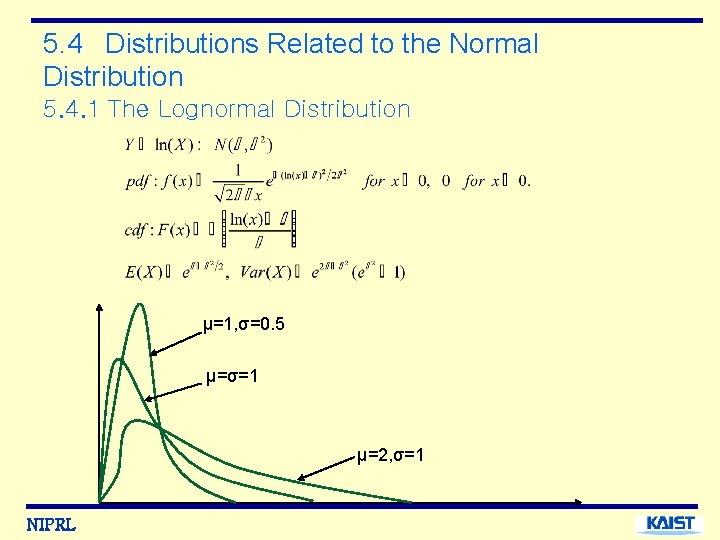
5. 4 Distributions Related to the Normal Distribution 5. 4. 1 The Lognormal Distribution μ=1, σ=0. 5 μ=σ=1 μ=2, σ=1 NIPRL

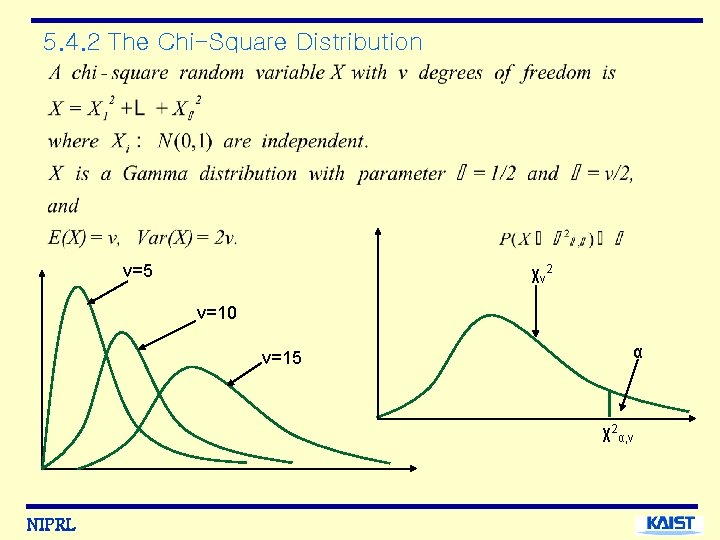
5. 4. 2 The Chi-Square Distribution ν=5 χν 2 ν=10 ν=15 α χ2α, ν NIPRL

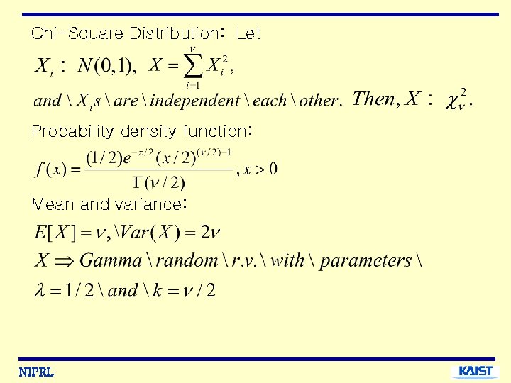
Chi-Square Distribution: Let Probability density function: Mean and variance: NIPRL

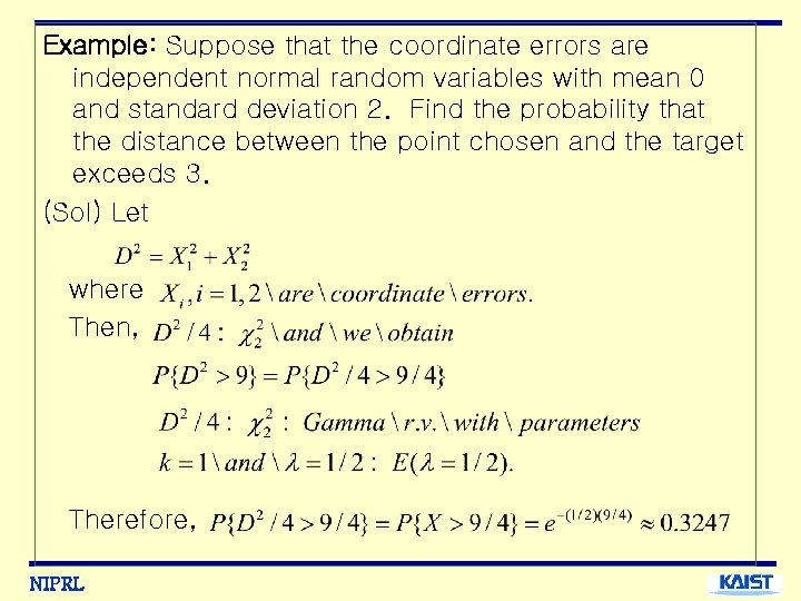
Example: Suppose that the coordinate errors are independent normal random variables with mean 0 and standard deviation 2. Find the probability that the distance between the point chosen and the target exceeds 3. (Sol) Let where Then, Therefore, NIPRL

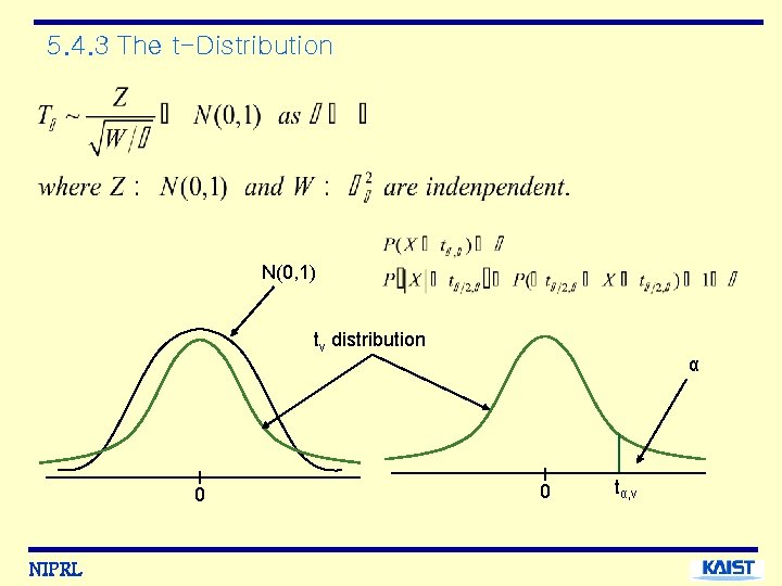
5. 4. 3 The t-Distribution N(0, 1) tv distribution 0 NIPRL α 0 tα, ν

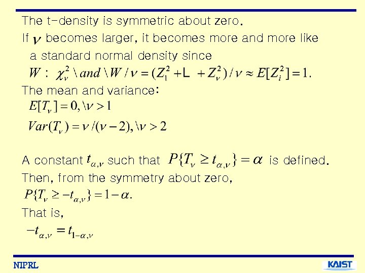
The t-density is symmetric about zero. If becomes larger, it becomes more and more like a standard normal density since The mean and variance: A constant such that Then, from the symmetry about zero, That is, NIPRL is defined.

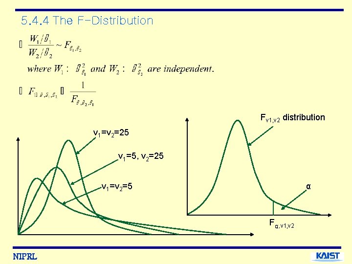
5. 4. 4 The F-Distribution Fν 1, ν 2 distribution ν 1=v 2=25 ν 1=5, v 2=25 ν 1=v 2=5 α Fα, ν 1, ν 2 NIPRL

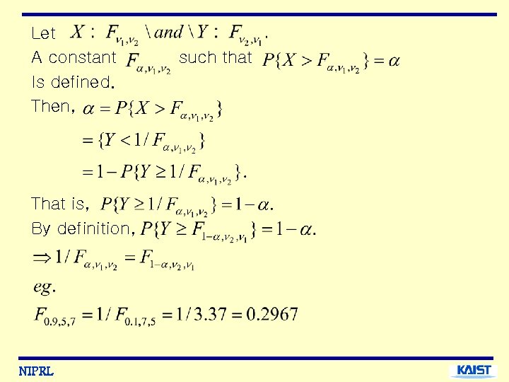
Let A constant Is defined. Then, That is, By definition, NIPRL such that

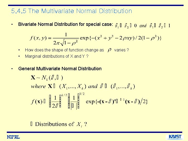
5. 4. 5 The Multivariate Normal Distribution • Bivariate Normal Distribution for special case: • • • How does the shape of function change as Marginal distributions of X and Y ? General Multivariate Normal Distribution NIPRL varies ?